Fit RV and Proper Motion Anomaly
In this example, we will fit an orbit model to a combination of radial velocity and Hipparcos-GAIA proper motion anomaly for the star $\epsilon$ Eridani. We will use some of the radial velocity data collated in Mawet et al 2019.
Radial velocity modelling is supported in Octofitter via the extension package OctofitterRadialVelocity. To install it, run pkg> add OctofitterRadialVelocity
Datasets from two different radial velocity insturments are included and modelled together with separate jitters and instrumental offsets.
using Octofitter, OctofitterRadialVelocity, Distributions, PlanetOrbits, CairoMakie

gaia_id = 5164707970261890560


planet_b = Planet(
    name="b",
    basis=Visual{KepOrbit},
    observations=[], # No planet astrometry is included since it has not yet been directly detected
    variables=@variables begin
        # For speed of example, we are fitting a circular orbit only.
        e = 0
        ω = 0.0
        mass ~ Uniform(0, 3)
        a ~ Uniform(3, 10)
        i ~ Sine()
        Ω ~ Uniform(0, 2pi)
        M = system.M
        τ ~ Uniform(0, 1.0)
        P = √(a^3/M)
        tp = τ*P*365.25 + 58849 # reference epoch for τ. Choose an MJD date near your data.
    end
)


# We will load in data from one RV instruments.
# We use `MarginalizedStarAbsoluteRVObs` instead of
# `StarAbsoluteRVObs` to automatically marginalize out
# the radial velocity zero point of each instrument, saving one parameter.
hires_data = OctofitterRadialVelocity.HIRES_rvs("HD22049")
rvlike_hires = MarginalizedStarAbsoluteRVObs(
    hires_data,
    name="HIRES",
    variables=@variables begin
        jitter ~ LogUniform(0.1, 100) # m/s
    end
)
MarginalizedStarAbsoluteRVObs Table with 4 columns and 117 rows:
epoch rv σ_rv inst_idx
┌────────────────────────────────
1 │ 55455.5 5.48 1.05 1
2 │ 55464.6 -10.52 1.02 1
3 │ 55468.6 8.43 0.95 1
4 │ 55486.5 -11.29 1.09 1
5 │ 55500.5 0.95 0.96 1
6 │ 55521.4 -12.6 0.98 1
7 │ 55542.4 -12.52 1.14 1
8 │ 55613.2 -0.15 0.97 1
9 │ 55790.6 3.34 0.89 1
10 │ 55791.6 -12.31 1.01 1
11 │ 55792.6 -17.59 0.86 1
12 │ 55794.6 -7.73 0.87 1
13 │ 55796.6 -2.02 0.81 1
14 │ 55797.6 -3.27 0.87 1
15 │ 55806.6 -3.42 0.99 1
16 │ 55808.6 -0.02 1.0 1
17 │ 55870.5 4.78 1.19 1
⋮ │ ⋮ ⋮ ⋮ ⋮We load the HGCA data for this target:
hgca_obs = HGCAInstantaneousObs(
    gaia_id=gaia_id,
    variables=@variables begin
        # Optional: flux ratio for luminous companions
        # fluxratio ~ Product([Uniform(0, 1), Uniform(0, 1), ])  # uncomment if needed for unresolved companions
    end
)
HGCAInstantaneousObs Table with 3 columns and 4 rows:
epoch meas inst
┌────────────────────
1 │ 48312.2 ra hip
2 │ 48423.4 dec hip
3 │ 57322.8 ra gaia
4 │ 57278.7 dec gaiaIn the interests of time, we use the HGCAInstantaneousObs approximation to speed up the computation. This parameter controls how the model smears out the simulated Gaia and Hipparcos measurements in time. For a real target, use HGCAObs instead which will simulate the Gaia and Hipparcos fits with greater fidelity.
sys = System(
    name="ϵEri",
    companions=[planet_b],
    observations=[hgca_obs, rvlike_hires],
    variables=@variables begin
        M ~ truncated(Normal(0.82, 0.02),lower=0.5, upper=1.5) # (Baines & Armstrong 2011).
        plx ~ gaia_plx(;gaia_id)
        pmra ~ Normal(-975, 10)
        pmdec ~ Normal(20,  10)
    end
)
# Build model
model = Octofitter.LogDensityModel(sys)
LogDensityModel for System ϵEri of dimension 10 and 121 epochs with fields .ℓπcallback and .∇ℓπcallback
Find good starting points and visualize the starting position + data:
init_chain = initialize!(model)
octoplot(model, init_chain, show_mass=true)
Now sample. You could use HMC via octofit or tempered sampling via octofit_pigeons. When using tempered sampling, make sure to start julia with julia --thread=auto. Each additional round doubles the number of posterior samples, so n_rounds=10 gives 1024 samples. You should adjust n_chains to be roughly double the Λ value printed out during sample, and n_chains_variational to be roughly double the Λ_var column.
using Pigeons
results, pt = octofit_pigeons(model, n_rounds=10, n_chains=10, n_chains_variational=0, explorer=SliceSampler());
[ Info: Sampler running with multiple threads : true
[ Info: Likelihood evaluated with multiple threads: false
─────────────────────────────────────────────────────────────────────────────────────────────────────────────
scans restarts Λ time(s) allc(B) log(Z₁/Z₀) min(α) mean(α) min(αₑ) mean(αₑ)
────────── ────────── ────────── ────────── ────────── ────────── ────────── ────────── ────────── ──────────
2 0 3.2 0.103 2.98e+06 -4.4e+04 0 0.645 1 1
4 0 4.93 0.105 3.16e+04 -2.11e+03 0 0.452 1 1
8 0 4.99 0.2 3.91e+04 -1.87e+03 0 0.445 1 1
16 0 5.64 0.398 5.97e+04 -899 2.29e-85 0.373 1 1
32 0 5.36 0.785 8.61e+04 -940 6.42e-120 0.404 1 1
64 9 1.45 1.88 2.48e+07 -811 0.541 0.838 1 1
128 18 1.55 3.64 4.31e+07 -810 0.722 0.828 1 1
256 43 1.52 7.58 8.59e+07 -810 0.776 0.831 1 1
512 92 1.57 14.3 1.71e+08 -811 0.797 0.826 1 1
1.02e+03 180 1.58 28.7 3.41e+08 -811 0.792 0.825 1 1
─────────────────────────────────────────────────────────────────────────────────────────────────────────────We can now plot the results with a multi-panel plot:
octoplot(model, results, show_mass=true)We can also plot just the RV curve from the maximum a-posteriori fit:
fig = Octofitter.rvpostplot(model, results)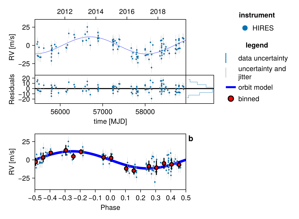
We can see what the visual orbit looks like for the maximum a-posteriori sample (note, we would need to run an optimizer to get the true MAP value; this is just the MCMC sample with higest posterior density):
i_max = argmax(results[:logpost][:])
fig = octoplot(
    model,
    results[i_max,:,:],
    # change the colour map a bit:
    colormap=Makie.cgrad([Makie.wong_colors()[1], "#FAFAFA"]),
    show_astrom=true,
    show_astrom_time=false,
    show_rv=false,
    show_pma=false,
    mark_epochs_mjd=[
        mjd("2037")
    ]
)
Label(fig[0,1], "Maximum a-posteriori orbit sample")
Makie.resize_to_layout!(fig)
fig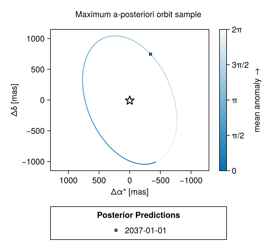
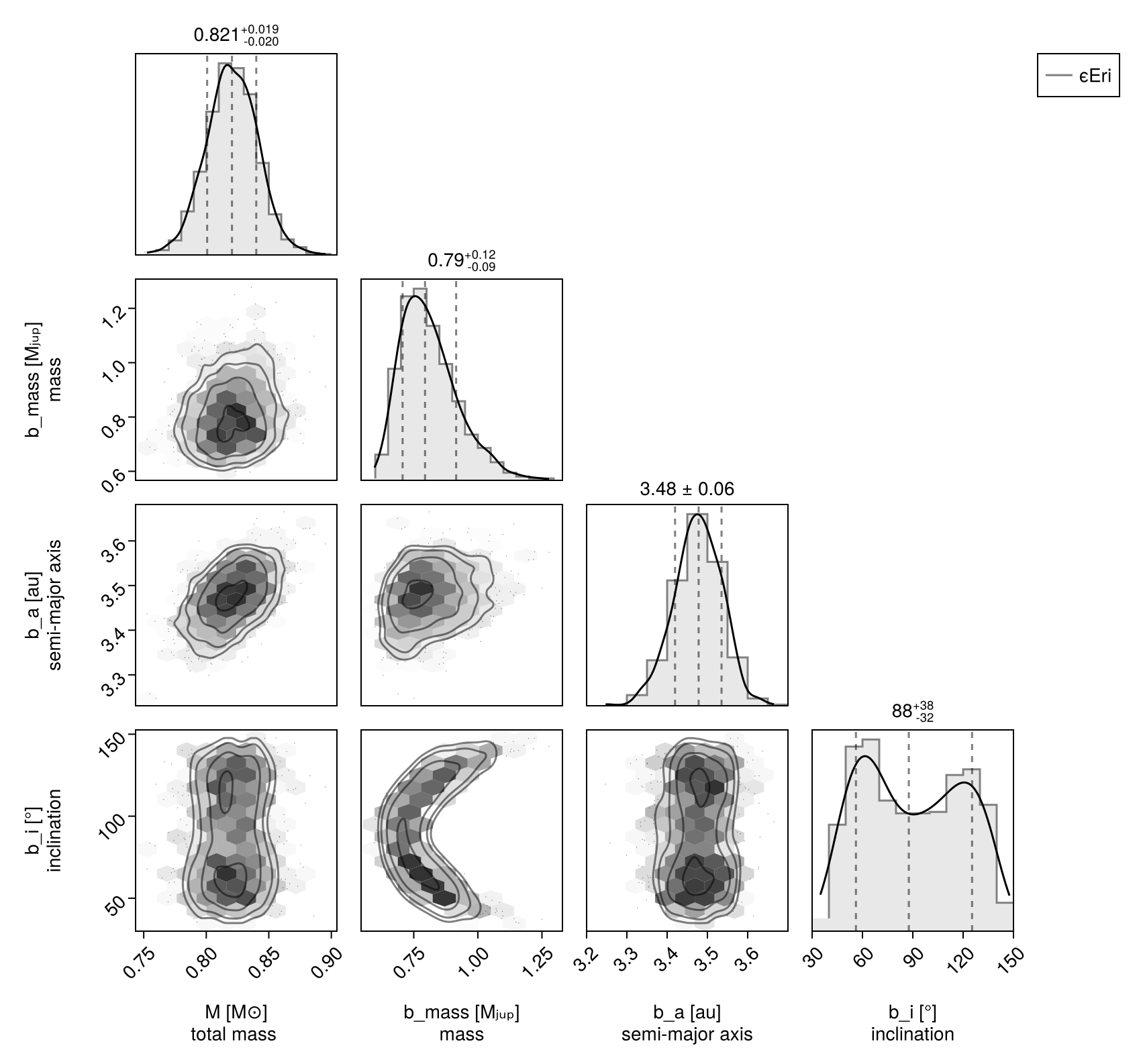
And a corner plot:
using CairoMakie, PairPlots
octocorner(model, results, small=true)