Observable-Based Priors
This tutorial shows how to fit an orbit to relative astrometry using the observable-based priors ofO'Neil et al. 2019. Please cite that paper if you use this functionality.
We will fit the same astrometry as in the previous tutorial, and just change our priors.
using Octofitter
using CairoMakie
using PairPlots
using Distributions

astrom_dat = Table(;
    epoch = [50000, 50120, 50240, 50360, 50480, 50600, 50720, 50840],
    ra    = [-494.4, -495.0, -493.7, -490.4, -485.2, -478.1, -469.1, -458.3],
    dec   = [-76.7, -44.9, -12.9, 19.1, 51.0, 82.8, 114.3, 145.3],
    σ_ra  = [12.6, 10.4, 9.9, 8.7, 8.0, 6.9, 5.8, 4.2],
    σ_dec = [12.6, 10.4, 9.9, 8.7, 8.0, 6.9, 5.8, 4.2],
    cor   = [0.2, 0.5, 0.1, -0.8, 0.3, -0.0, 0.1, -0.2]
)

astrom_obs = PlanetRelAstromObs(
    astrom_dat,
    name = "obs_prior_example",
    variables = @variables begin
        # Fixed values for this example - could be free variables:
        jitter = 0        # mas [could use: jitter ~ Uniform(0, 10)]
        northangle = 0    # radians [could use: northangle ~ Normal(0, deg2rad(1))]
        platescale = 1    # relative [could use: platescale ~ truncated(Normal(1, 0.01), lower=0)]
    end
)
# We wrap the likelihood in this prior
obs_pri_astrom_obs = ObsPriorAstromONeil2019(astrom_obs)

planet_b = Planet(
    name="b",
    basis=Visual{KepOrbit},
    # NOTE! We only provide the wrapped obs_pri_astrom_obs
    observations=[obs_pri_astrom_obs],
    variables=@variables begin
        M = system.M
        e ~ Uniform(0.0, 0.5)
        i ~ Sine()
        ω ~ UniformCircular()
        Ω ~ UniformCircular()
        # Results will be sensitive to the prior on period
        P ~  LogUniform(0.1, 150) # Period, years
        a = ∛(M * P^2)
        θ_x ~ Normal()
        θ_y ~ Normal()
        θ = atan(θ_y, θ_x)
        tp = θ_at_epoch_to_tperi(θ, 50420; M, e, a, i, ω, Ω)
    end
)

sys = System(
    name="TutoriaPrime",
    companions=[planet_b],
    observations=[],
    variables=@variables begin
        M ~ truncated(Normal(1.2, 0.1), lower=0.1)
        plx ~ truncated(Normal(50.0, 0.02), lower=0.1)
    end
)

model = Octofitter.LogDensityModel(sys)
LogDensityModel for System TutoriaPrime of dimension 11 and 10 epochs with fields .ℓπcallback and .∇ℓπcallback
Initialize the model starting points and confirm the data are entered correctly:
init_chain = initialize!(model,)
octoplot(model, init_chain)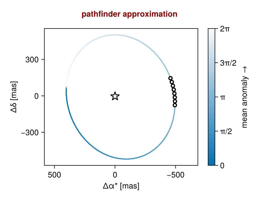
Now run the fit:
results_obspri = octofit(model,iterations=5000,)Chains MCMC chain (5000×33×1 Array{Float64, 3}):
Iterations = 1:1:5000
Number of chains = 1
Samples per chain = 5000
Wall duration = 10.39 seconds
Compute duration = 10.39 seconds
parameters = M, plx, b_e, b_i, b_ωx, b_ωy, b_Ωx, b_Ωy, b_P, b_θ_x, b_θ_y, b_ω, b_Ω, b_M, b_a, b_θ, b_tp, b_obspri_obs_prior_example_jitter, b_obspri_obs_prior_example_northangle, b_obspri_obs_prior_example_platescale
internals = n_steps, is_accept, acceptance_rate, hamiltonian_energy, hamiltonian_energy_error, max_hamiltonian_energy_error, tree_depth, numerical_error, step_size, nom_step_size, is_adapt, loglike, logpost, tree_depth, numerical_error
Use `describe(chains)` for summary statistics and quantiles.
Plot the MCMC results:
octoplot(model, results_obspri)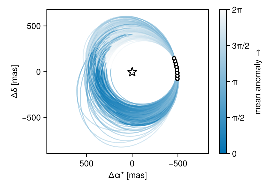
Compare this with the previous fit using uniform priors:
octoplot(model_with_uniform_priors, results_unif_pri)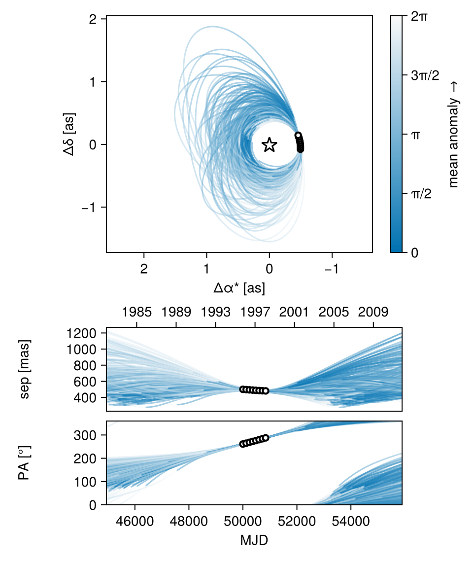
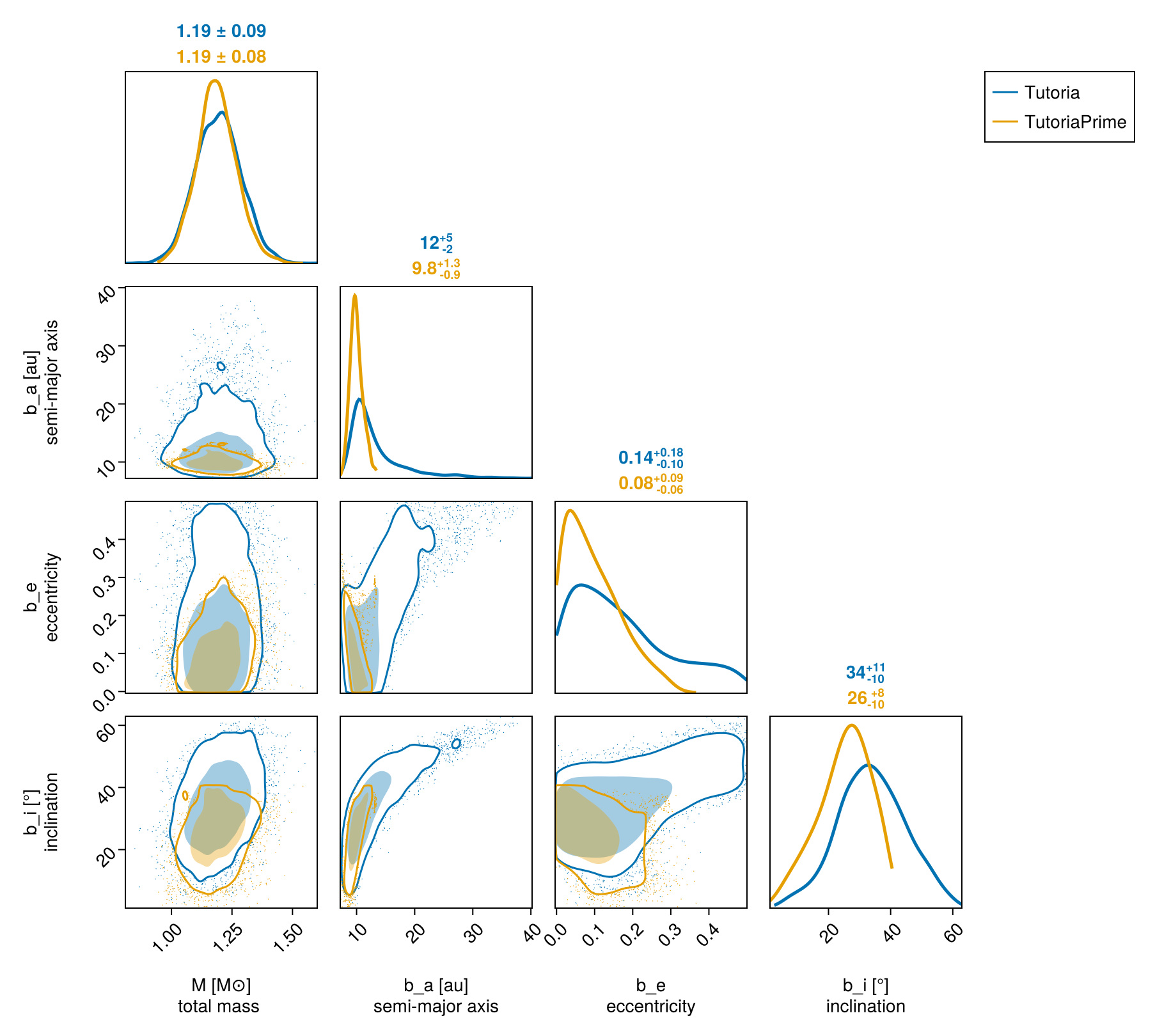
We can compare the results in a corner plot:
octocorner(model,results_unif_pri,results_obspri,small=true)