Fit Gaussian Process
This example shows how to fit a Gaussian process to model stellar activity in RV data. It continues from Basic RV Fit.
Radial velocity modelling is supported in Octofitter via the extension package OctofitterRadialVelocity. To install it, run pkg> add OctofitterRadialVelocity
There are two different GP packages supported by OctofitterRadialVelocity: AbstractGPs, and Celerite. Important note: Celerite.jl does not support Julia 1.0+, so we currently bundle a fork that has been patched to work. When / if Celerite.jl is updated we will switch back to the public package.
GP models are significantly more computationally expensive than non-GP models. Plan for longer sampling times when using Gaussian processes.
For this example, we will fit the orbit of the planet K2-131 to perform the same fit as in the RadVel Gaussian Process Fitting tutorial.
We will use the following packages:
using Octofitter
using OctofitterRadialVelocity
using PlanetOrbits
using CairoMakie
using PairPlots
using CSV
using DataFrames
using Distributions
We will pick up from our tutorial Basic RV Fit with the data already downloaded and available as a table called rv_dat:
rv_file = download("https://raw.githubusercontent.com/California-Planet-Search/radvel/master/example_data/k2-131.txt")
rv_dat_raw = CSV.read(rv_file, DataFrame, delim=' ')
rv_dat = DataFrame();
rv_dat.epoch = jd2mjd.(rv_dat_raw.time)
rv_dat.rv = rv_dat_raw.mnvel
rv_dat.σ_rv = rv_dat_raw.errvel
tels = sort(unique(rv_dat_raw.tel))
2-element Vector{InlineStrings.String7}:
"harps-n"
"pfs"Gaussian Process Fit with AbstractGPs
Let us now add a Gaussian process to model stellar activity. This should improve the fit.
We start by writing a function that creates a Gaussian process kernel from a set of system parameters. We will create a quasi-periodic kernel. We provide this function as an arugment gaussian_process to the likelihood constructor:
using AbstractGPs

gp_explength_mean = 9.5*sqrt(2.) # sqrt(2)*tau in Dai+ 2017 [days]
gp_explength_unc = 1.0*sqrt(2.)
gp_perlength_mean = sqrt(1. /(2. *3.32)) # sqrt(1/(2*gamma)) in Dai+ 2017
gp_perlength_unc = 0.019
gp_per_mean = 9.64 # T_bar in Dai+ 2017 [days]
gp_per_unc = 0.12

rvlike_harps = StarAbsoluteRVObs(
    rv_dat[rv_dat_raw.tel .== "harps-n",:],
    name="harps-n",
    gaussian_process = θ_obs -> GP(
        θ_obs.η_1^2 *
        (SqExponentialKernel() ∘ ScaleTransform(1/(θ_obs.η_2))) *
        (PeriodicKernel(r=[θ_obs.η_4]) ∘ ScaleTransform(1/(θ_obs.η_3)))
    ),
    # Note: variables= must come last
    variables=@variables begin
        offset ~ Normal(-6693,100) # m/s
        jitter ~ LogUniform(0.1,100) # m/s
        # Add priors on GP kernel hyper-parameters.
        η_1 ~ truncated(Normal(25,10),lower=0.1,upper=100)
        # Important: ensure the period and exponential length scales
        # have physically plausible lower and upper limits to avoid poor numerical conditioning
        η_2 ~ truncated(Normal(gp_explength_mean,gp_explength_unc),lower=5,upper=100)
        η_3 ~ truncated(Normal(gp_per_mean,1),lower=2, upper=100)
        η_4 ~ truncated(Normal(gp_perlength_mean,gp_perlength_unc),lower=0.2, upper=10)
    end
)
rvlike_pfs = StarAbsoluteRVObs(
    rv_dat[rv_dat_raw.tel .== "pfs",:],
    name="pfs",
    gaussian_process = θ_obs -> GP(
        θ_obs.η_1^2 *
        (SqExponentialKernel() ∘ ScaleTransform(1/(θ_obs.η_2))) *
        (PeriodicKernel(r=[θ_obs.η_4]) ∘ ScaleTransform(1/(θ_obs.η_3)))
    ),
    # Note: variables= must come last
    variables=@variables begin
        offset ~ Normal(0,100) # m/s
        jitter ~ LogUniform(0.1,100) # m/s
        # Add priors on GP kernel hyper-parameters.
        η_1 ~ truncated(Normal(25,10),lower=0.1,upper=100)
        # Important: ensure the period and exponential length scales
        # have physically plausible lower and upper limits to avoid poor numerical conditioning
        η_2 ~ truncated(Normal(gp_explength_mean,gp_explength_unc),lower=5,upper=100)
        η_3 ~ truncated(Normal(gp_per_mean,1),lower=2, upper=100)
        η_4 ~ truncated(Normal(gp_perlength_mean,gp_perlength_unc),lower=0.2, upper=10)
    end
)
## No change to the rest of the model

planet_1 = Planet(
    name="b",
    basis=RadialVelocityOrbit,
    observations=[],
    variables=@variables begin
        e = 0
        ω = 0.0
        # To match RadVel, we set a prior on Period and calculate semi-major axis from it
        P ~ truncated(
            Normal(0.3693038/365.256360417, 0.0000091/365.256360417),
            lower=0.0001
        )
        M = system.M
        a = cbrt(M * P^2) # note the equals sign.
        τ ~ UniformCircular(1.0)
        tp = τ*P*365.256360417 + 57782 # reference epoch for τ. Choose an MJD date near your data.
        # minimum planet mass [jupiter masses]. really m*sin(i)
        mass ~ LogUniform(0.001, 10)
    end
)

sys = System(
    name = "k2_132",
    companions=[planet_1],
    observations=[rvlike_harps, rvlike_pfs],
    variables=@variables begin
        M ~ truncated(Normal(0.82, 0.02),lower=0.1) # (Baines & Armstrong 2011).
    end
)

model = Octofitter.LogDensityModel(sys)
LogDensityModel for System k2_132 of dimension 17 and 71 epochs with fields .ℓπcallback and .∇ℓπcallback
Note that the two instruments do not need to use the same Gaussian process kernels, nor the same hyper parameter names.
Tip: If you want the instruments to share the Gaussian process kernel hyper parameters, move the variables up to the system's @variables block, and forward them to the observation variables block e.g. η₁ = system.η₁, η₂ = system.η₂.
Initialize the starting points, and confirm the data are entered correcly:
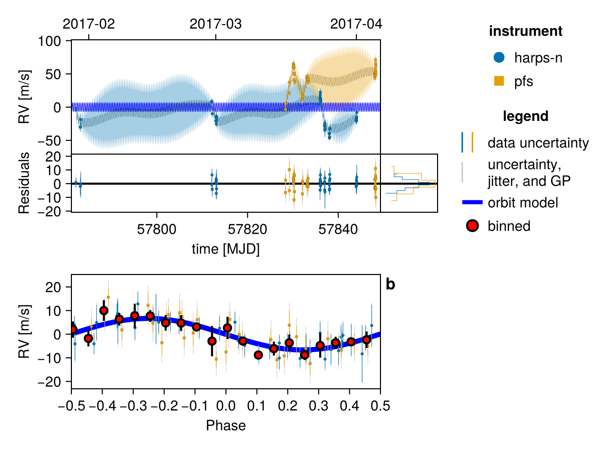
init_chain = initialize!(model)
fig = Octofitter.rvpostplot(model, init_chain)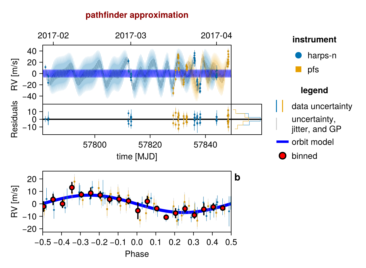
Sample from the model using MCMC (the no U-turn sampler)
# Seed the random number generator
using Random
rng = Random.Xoshiro(0)

chain = octofit(
    rng, model,
    adaptation = 100,
    iterations = 100,
)
Chains MCMC chain (100×36×1 Array{Float64, 3}):
Iterations = 1:1:100
Number of chains = 1
Samples per chain = 100
Wall duration = 1029.7 seconds
Compute duration = 1029.7 seconds
parameters = M, harps_n_offset, harps_n_jitter, harps_n_η_1, harps_n_η_2, harps_n_η_3, harps_n_η_4, pfs_offset, pfs_jitter, pfs_η_1, pfs_η_2, pfs_η_3, pfs_η_4, b_P, b_τx, b_τy, b_mass, b_τ, b_e, b_ω, b_M, b_a, b_tp
internals = n_steps, is_accept, acceptance_rate, hamiltonian_energy, hamiltonian_energy_error, max_hamiltonian_energy_error, tree_depth, numerical_error, step_size, nom_step_size, is_adapt, loglike, logpost, tree_depth, numerical_error
Use `describe(chains)` for summary statistics and quantiles.
For real data, we would want to increase the adaptation and iterations to about 1000 each.
Plot one sample from the results:
fig = Octofitter.rvpostplot(model, chain) # saved to "k2_132-rvpostplot.png"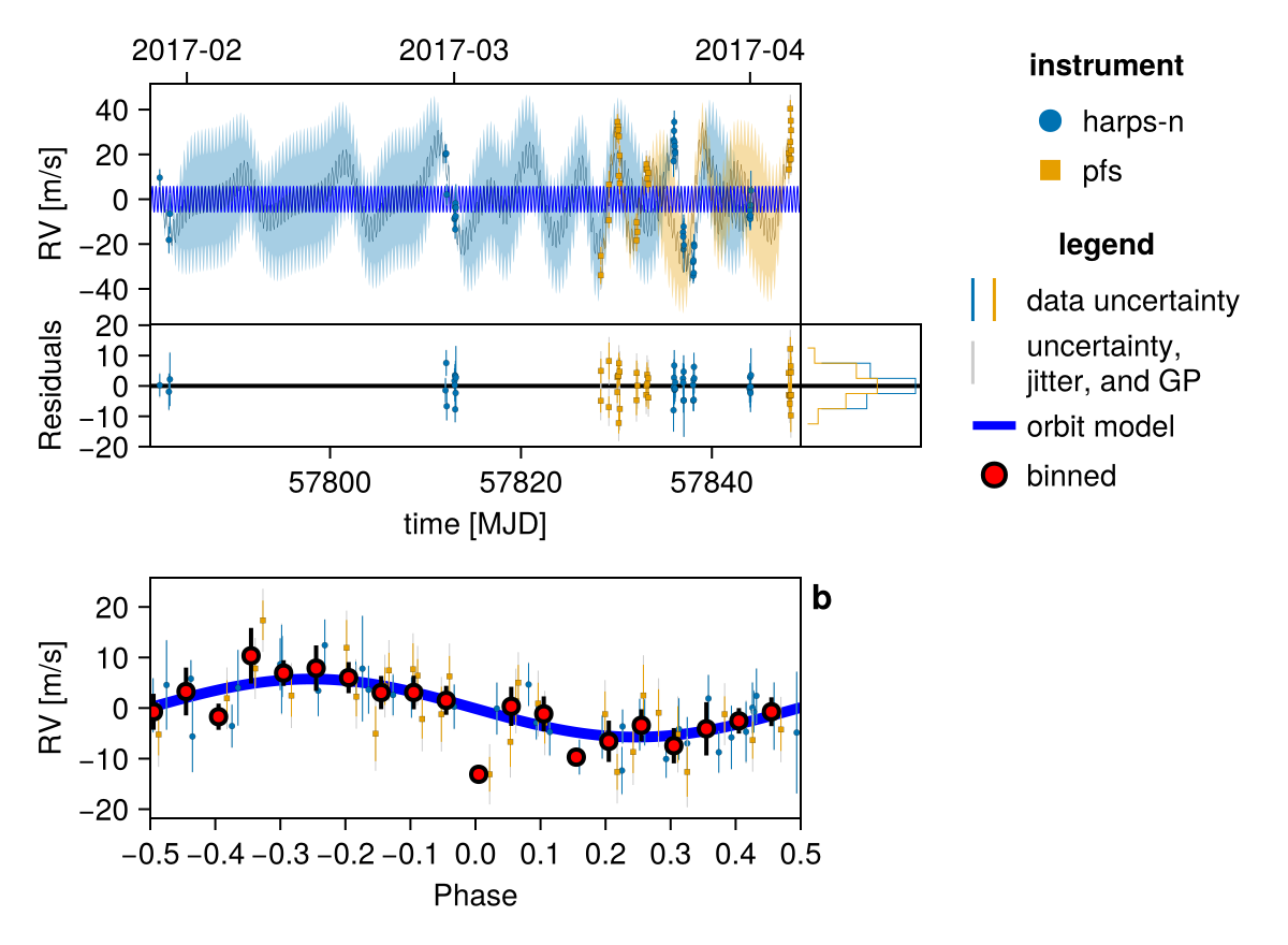
Plot many samples from the results:
fig = octoplot(
    model,
    chain,
    # Some optional tweaks to the appearance:
    N=50, # only plot 50 samples
    figscale=1.5, # make it larger
    alpha=0.05, # make each sample more transparent
    colormap="#0072b2",
) # saved to "k2_132-plot-grid.png"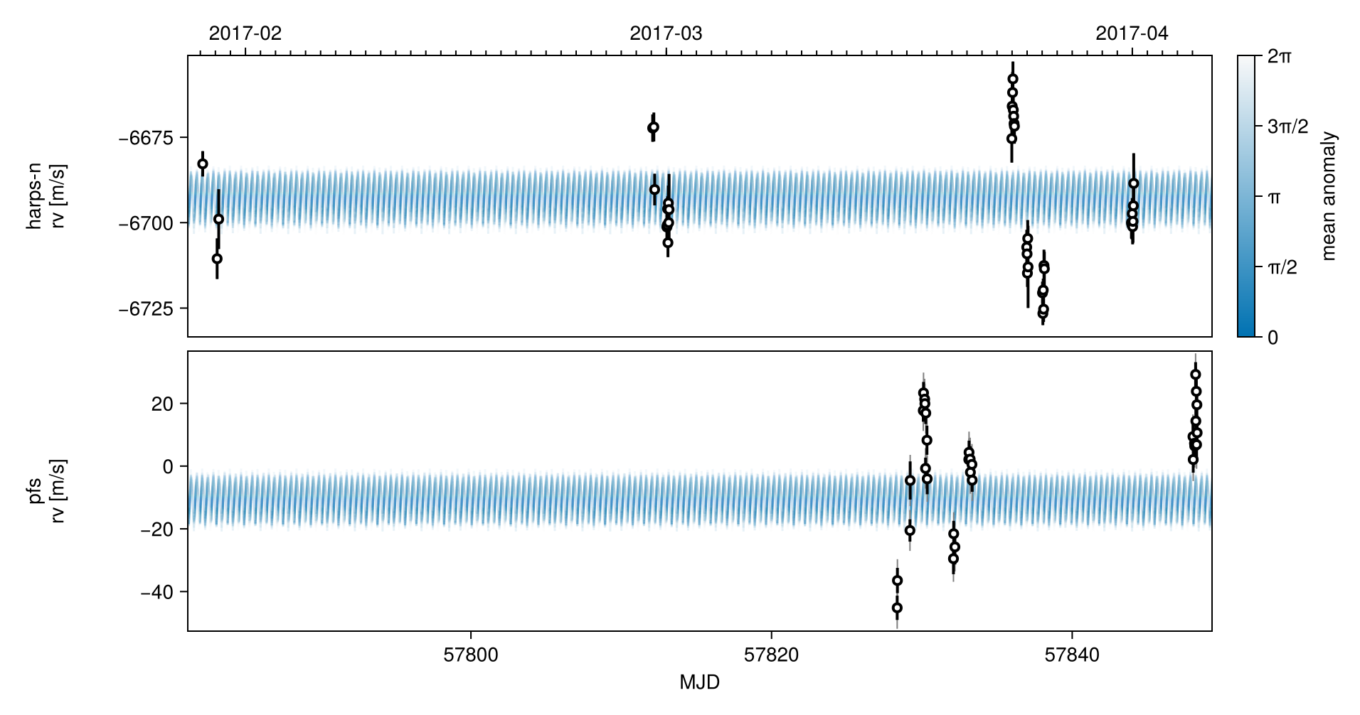
Corner plot:
octocorner(model, chain, small=true) # saved to "k2_132-pairplot-small.png"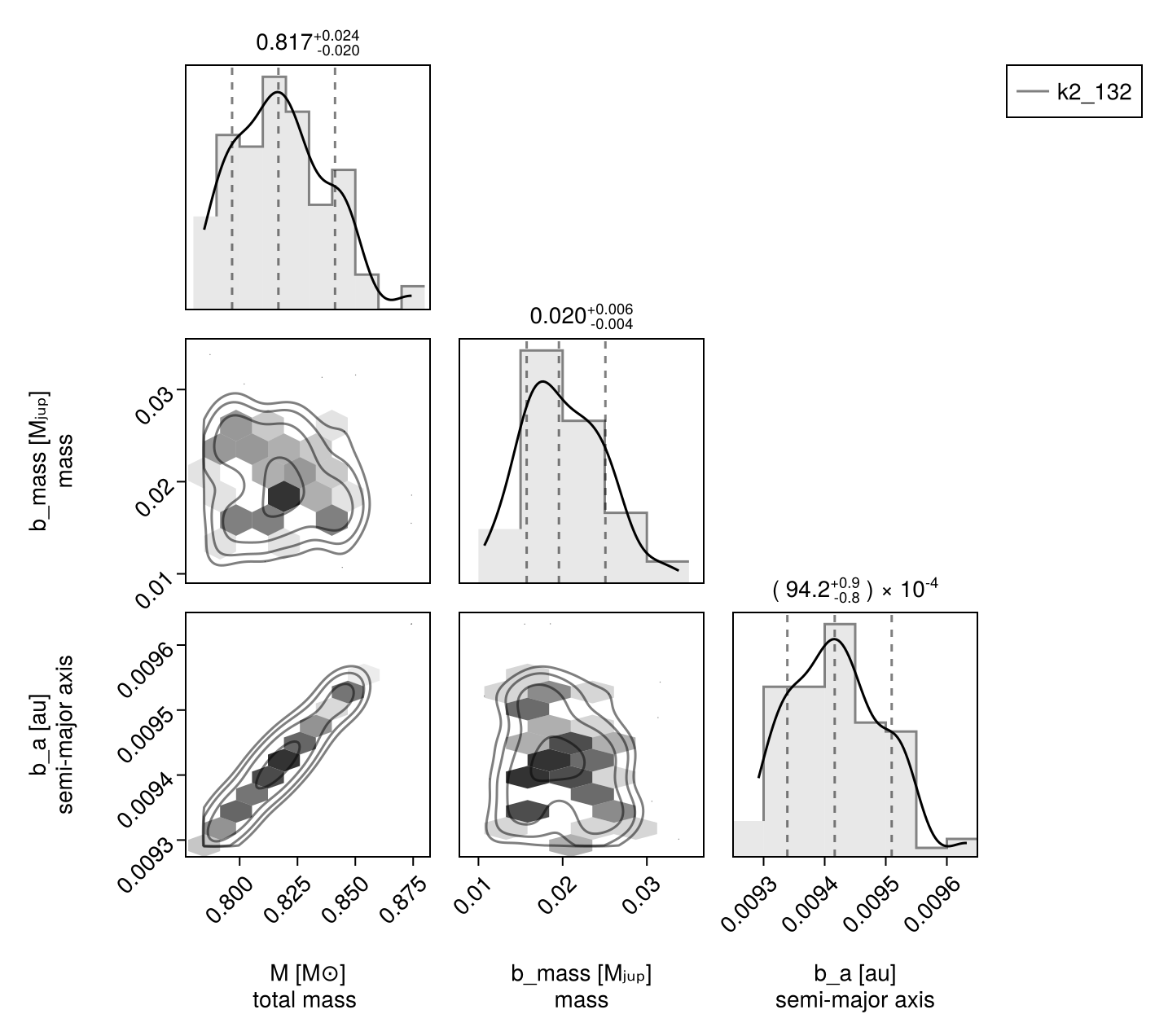
Gaussian Process Fit with Celerite
We now demonstrate an approximate quasi-static kernel implemented using Celerite. For the class of kernels supported by Celerite, the performance scales much better with the number of data points. This makes it a good choice for modelling large RV datasets.
Make sure that you type using OctofitterRadialVelocity.Celerite and not using Celerite. Celerite.jl does not support Julia 1.0+, so we currently bundle a fork that has been patched to work. When / if Celerite.jl is updated we will switch back to the public package.
using OctofitterRadialVelocity.Celerite

rvlike_harps = StarAbsoluteRVObs(
    rv_dat[rv_dat_raw.tel .== "harps-n",:],
    name="harps-n",
    gaussian_process = θ_obs -> Celerite.CeleriteGP(
        Celerite.RealTerm(
            #=log_a=# log(θ_obs.B*(1+θ_obs.C)/(2+θ_obs.C)),
            #=log_c=# log(1/θ_obs.L)
        ) + Celerite.ComplexTerm(
            #=log_a=#  log(θ_obs.B/(2+θ_obs.C)),
            #=log_b=#  -Inf,
            #=log_c=#  log(1/θ_obs.L),
            #=log_d=#  log(2pi/θ_obs.Prot)
        )
    ),
    # Note: variables= must come last
    variables=@variables begin
        offset ~ Normal(-6693,100) # m/s
        jitter ~ LogUniform(0.1,100) # m/s
        # Add priors on GP kernel hyper-parameters.
        B ~ Uniform(0.00001, 2000000)
        C ~ Uniform(0.00001, 200)
        L ~ Uniform(2, 200)
        Prot ~ Uniform(8.5, 20)#Uniform(0, 20)
    end
)
rvlike_pfs = StarAbsoluteRVObs(
    rv_dat[rv_dat_raw.tel .== "pfs",:],
    name="pfs",
    gaussian_process = θ_obs -> Celerite.CeleriteGP(
        Celerite.RealTerm(
            #=log_a=# log(θ_obs.B*(1+θ_obs.C)/(2+θ_obs.C)),
            #=log_c=# log(1/θ_obs.L)
        ) + Celerite.ComplexTerm(
            #=log_a=#  log(θ_obs.B/(2+θ_obs.C)),
            #=log_b=#  -Inf,
            #=log_c=#  log(1/θ_obs.L),
            #=log_d=#  log(2pi/θ_obs.Prot)
        )
    ),
    # Note: variables= must come last
    variables=@variables begin
        offset ~ Normal(0,100) # m/s
        jitter ~ LogUniform(0.1,100) # m/s
        # Add priors on GP kernel hyper-parameters.
        B ~ Uniform(0.00001, 2000000)
        C ~ Uniform(0.00001, 200)
        L ~ Uniform(2, 200)
        Prot ~ Uniform(8.5, 20)#Uniform(0, 20)
    end
)

## No change to the rest of the model

planet_1 = Planet(
    name="b",
    basis=RadialVelocityOrbit,
    observations=[],
    variables=@variables begin
        e = 0
        ω = 0.0
        # To match RadVel, we set a prior on Period and calculate semi-major axis from it
        P ~ truncated(
            Normal(0.3693038/365.256360417, 0.0000091/365.256360417),
            lower=0.0001
        )
        M = system.M
        a = cbrt(M * P^2) # note the equals sign.
        τ ~ UniformCircular(1.0)
        tp = τ*P*365.256360417 + 57782 # reference epoch for τ. Choose an MJD date near your data.
        # minimum planet mass [jupiter masses]. really m*sin(i)
        mass ~ LogUniform(0.001, 10)
    end
)

sys = System(
    name = "k2_132",
    companions=[planet_1],
    observations=[rvlike_harps, rvlike_pfs],
    variables=@variables begin
        M ~ truncated(Normal(0.82, 0.02),lower=0.1) # (Baines & Armstrong 2011).
    end
)

using DifferentiationInterface
using FiniteDiff
model = Octofitter.LogDensityModel(sys, autodiff=AutoFiniteDiff())
LogDensityModel for System k2_132 of dimension 17 and 71 epochs with fields .ℓπcallback and .∇ℓπcallback
The Celerite implementation doesn't support our default autodiff-backend (ForwardDiff.jl), so we disable autodiff by setting it to finite differences, and then using the Pigeons slice sampler which doesn't require gradients or (B) use Enzyme autodiff,
Initialize the starting points, and confirm the data are entered correcly:
init_chain = initialize!(model)
fig = Octofitter.rvpostplot(model, init_chain)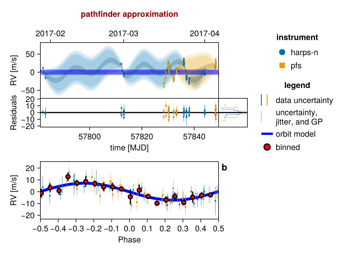
using Pigeons
chain, pt = octofit_pigeons(model, n_rounds=7)
fig = Octofitter.rvpostplot(model, chain)