Fit Relative RV Data
Octofitter includes support for fitting relative radial velocity data. Currently this is only tested with a single companion. Please open an issue if you would like to fit multiple companions simultaneously.
The convention we adopt is that positive relative radial velocity is the velocity of the companion (exoplanets) minus the velocity of the host (star).
To fit relative RV data, start by creating a likelihood object:
using Octofitter
using OctofitterRadialVelocity
using CairoMakie
using Distributions

rv_dat_1 = Table(
    epoch=55000:100:57400,
    rv = [
         -24022.74
        -18571.33
        14221.56
        26076.89
        -459.26
        -26319.26
        -13430.96
        19230.96
        23580.26
        -6786.28
        -27161.78
        -7548.58
        23177.95
        19780.94
        -12738.39
        -26503.74
        -1249.19
        25844.47
        14888.83
        -17986.76
        -24381.49
        5119.22
        27083.2
        9174.18
        -22241.45
    ],
    # Hint! Type as \sigma + <TAB>
    σ_rv= fill(15000.0, 25),
)


rel_rv_obs = PlanetRelativeRVObs(
    rv_dat_1,
    name="simulated data",
    variables = @variables begin
        jitter ~ LogUniform(0.1, 1000) # m/s
    end
)
PlanetRelativeRVObs Table with 3 columns and 25 rows:
epoch rv σ_rv
┌─────────────────────────
1 │ 55000 -24022.7 15000.0
2 │ 55100 -18571.3 15000.0
3 │ 55200 14221.6 15000.0
4 │ 55300 26076.9 15000.0
5 │ 55400 -459.26 15000.0
6 │ 55500 -26319.3 15000.0
7 │ 55600 -13431.0 15000.0
8 │ 55700 19231.0 15000.0
9 │ 55800 23580.3 15000.0
10 │ 55900 -6786.28 15000.0
11 │ 56000 -27161.8 15000.0
12 │ 56100 -7548.58 15000.0
13 │ 56200 23178.0 15000.0
14 │ 56300 19780.9 15000.0
15 │ 56400 -12738.4 15000.0
16 │ 56500 -26503.7 15000.0
17 │ 56600 -1249.19 15000.0
⋮ │ ⋮ ⋮ ⋮See the standard radial velocity tutorial for examples on how this data can be loaded from a CSV file.
The relative RV likelihood does not incorporate an instrument-specific RV offset. A jitter parameter can still be specified in the likelihood's @variables block, as can parameters for a gaussian process model of stellar noise. Currently only a single instrument jitter parameter is supported. If you need to model relative radial velocities from multiple instruments with different jitters, please open an issue on GitHub.
Next, create a planet and system model, attaching the relative rv likelihood to the planet.
planet_1 = Planet(
    name="b",
    basis=RadialVelocityOrbit,
    observations=[rel_rv_obs],
    variables=@variables begin
        M ~ truncated(Normal(1.2, 0.1), lower=0.1) # total mass in solar masses
        a ~ Uniform(0,10)
        e ~ Uniform(0.0, 0.5)
        i ~ Sine()
        ω ~ Uniform(0, 2pi)
        Ω ~ Uniform(0, 2pi)
        τ ~ Uniform(0, 1.0)
        P = √(a^3/M)
        tp = τ*P*365.25 + 60000 # reference epoch for τ. Choose an MJD date near your data.

    end
)
sys = System(
    name = "Example-System",
    companions=[planet_1],
    observations=[],
    variables=@variables begin
    end
)

model = Octofitter.LogDensityModel(sys)
LogDensityModel for System Example-System of dimension 8 and 25 epochs with fields .ℓπcallback and .∇ℓπcallback
Initialize the model and verify starting point
init_chain = initialize!(model)

octoplot(model, init_chain)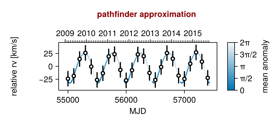
using Random
rng = Random.Xoshiro(123)
chain = octofit(rng, model)
Chains MCMC chain (1000×23×1 Array{Float64, 3}):
Iterations = 1:1:1000
Number of chains = 1
Samples per chain = 1000
Wall duration = 3.99 seconds
Compute duration = 3.99 seconds
parameters = b_M, b_a, b_e, b_i, b_ω, b_Ω, b_τ, b_P, b_tp, b_simulated_data_jitter
internals = n_steps, is_accept, acceptance_rate, hamiltonian_energy, hamiltonian_energy_error, max_hamiltonian_energy_error, tree_depth, numerical_error, step_size, nom_step_size, is_adapt, loglike, logpost, tree_depth, numerical_error
Use `describe(chains)` for summary statistics and quantiles.
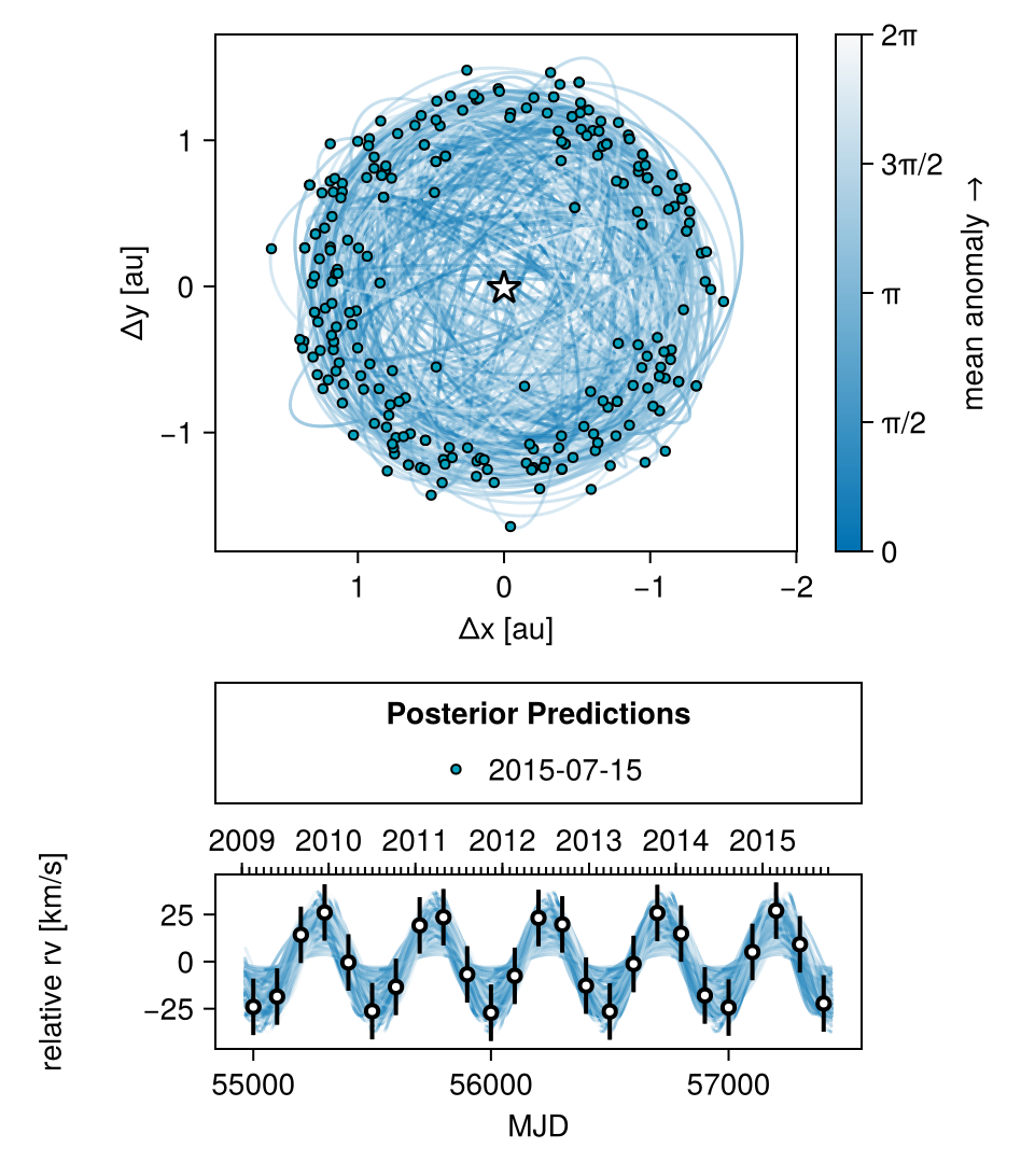
octoplot(model, chain, show_physical_orbit=true, mark_epochs_mjd=[mjd("2015-07-15")])