Basic Astrometry Fit
Here is a worked example of a one-planet model fit to relative astrometry (positions measured between the planet and the host star).
Start by loading the Octofitter and Distributions packages:
using Octofitter, DistributionsSpecifying the data
We will create a likelihood object to contain our relative astrometry data. We can specify this data in several formats. It can be listed in the code or loaded from a file (eg. a CSV file, FITS table, or SQL database). You can use any Julia table object.
astrom_dat_1 = Table(;
    epoch= [50000,  50120, 50240, 50360,50480, 50600, 50720, 50840,], # MJD (days)
    ra   = [-505.764, -502.57, -498.209, -492.678,-485.977, -478.11, -469.08, -458.896,], # mas
    dec  = [-66.9298, -37.4722, -7.92755, 21.6356, 51.1472,  80.5359,  109.729,  138.651, ], # mas
    # Tip! Type this as \sigma + <TAB key>!
    σ_ra = [10.0, 10.0, 10.0, 10.0, 10.0, 10.0, 10.0, 10.0, ],  # mas
    σ_dec = [10.0, 10.0, 10.0, 10.0, 10.0, 10.0, 10.0, 10.0, ], # mas
    cor =  [0.0, 0.0, 0.0, 0.0, 0.0, 0.0, 0.0, 0.0, ]
)
astrom_obs_1 = PlanetRelAstromObs(astrom_dat_1, name="relastrom")
PlanetRelAstromObs Table with 6 columns and 8 rows:
epoch ra dec σ_ra σ_dec cor
┌────────────────────────────────────────────
1 │ 50000 -505.764 -66.9298 10.0 10.0 0.0
2 │ 50120 -502.57 -37.4722 10.0 10.0 0.0
3 │ 50240 -498.209 -7.92755 10.0 10.0 0.0
4 │ 50360 -492.678 21.6356 10.0 10.0 0.0
5 │ 50480 -485.977 51.1472 10.0 10.0 0.0
6 │ 50600 -478.11 80.5359 10.0 10.0 0.0
7 │ 50720 -469.08 109.729 10.0 10.0 0.0
8 │ 50840 -458.896 138.651 10.0 10.0 0.0In Octofitter, epoch is always the modified Julian date (measured in days). If you're not sure what this is, you can get started by just putting in arbitrary time offsets measured in days.
In this case, we specified ra and dec offsets in milliarcseconds. We could instead specify sep (projected separation) in milliarcseconds and pa in radians. You cannot mix the two formats in a single PlanetRelAstromObs but you can create two different likelihood objects, one for each format, and add them both to your model:
You can also specify it in separation (mas) and positon angle (rad):
astrom_dat_2 = Table(
    epoch = [42000, ], # MJD
    sep = [505.7637580573554, ], # mas
    pa = [deg2rad(24.1), ], # radians
    # Tip! Type this as \sigma + <TAB key>!
    σ_sep = [70, ],
    σ_pa = [deg2rad(10.2), ],
)
astrom_obs_2 = PlanetRelAstromObs(astrom_dat_2, name="relastrom2")
PlanetRelAstromObs Table with 5 columns and 1 row:
epoch sep pa σ_sep σ_pa
┌──────────────────────────────────────────
1 │ 42000 505.764 0.420624 70 0.178024Advanced Options
You can group your data in different likelihood objects, each with their own instrument name. Each group can have its own platescale, northangle, and astrometric jitter variables for modelling instrument-specific systematics.
astrom_obs_1 = PlanetRelAstromObs(
    astrom_dat_1,
    name = "GPI astrom",
    variables = @variables begin
        jitter ~ Uniform(0, 10) # mas [optional]
        northangle ~ Normal(0, deg2rad(1)) # radians of offset [optional]
        platescale ~ truncated(Normal(1, 0.01), lower=0) # 1% relative platescale uncertainty
    end
)

astrom_obs_2 = PlanetRelAstromObs(
    astrom_dat_2,
    name = "SPHERE astrom",
    variables = @variables begin
        jitter ~ Uniform(0, 10) # mas [optional]
        northangle ~ Normal(0, deg2rad(1)) # radians of offset [optional]
        platescale ~ truncated(Normal(1, 0.01), lower=0) # 1% relative platescale uncertainty
    end
)
In Octofitter, epoch is always the modified Julian date (measured in days). If you're not sure what this is, you can get started by just putting in arbitrary time offsets measured in days.
In this case, we specified ra and dec offsets in milliarcseconds. We could instead specify sep (projected separation) in milliarcseconds and pa in radians. You cannot mix the two formats in a single PlanetRelAstromObs but you can create two different likelihood objects, one for each format.
Creating a planet
We now create our first planet model. Let's name it planet b. The name of the planet will be used in the output results.
In Octofitter, we specify planet and system models using a "probabilistic programming language". Quantities with a ~ are random variables. The distributions on the right hand sides are priors. You must specify a proper prior for any quantity which is allowed to vary.
We now create a planet model incorporating our likelihoods and specify our priors.
planet_1 = Planet(
    name="b",
    basis=Visual{KepOrbit},
    observations=[astrom_obs_1, astrom_obs_2],
    variables=@variables begin
        plx = system.plx
        M ~ truncated(Normal(1.2, 0.1), lower=0.1)
        a ~ Uniform(0, 100)
        e ~ Uniform(0.0, 0.5)
        i ~ Sine()
        ω ~ UniformCircular()
        Ω ~ UniformCircular()
        θ ~ UniformCircular()
        tp = θ_at_epoch_to_tperi(θ, 50420; M, e, a, i, ω, Ω)
    end
)name: Try to give your companion a short name consisting only of letters and/or trailing numbers.
basis: Visual{KepOrbit} is the type of orbit parameterization. There are several options available in the PlanetOrbits.jl documentation. The basis controls how how the orbit is calculated and what variables must be supplied.
likelihoods: A list of zero or more likelihood objects containing our data
variables: The variables block specifies our priors. You must supply every variable needed by your chosen basis, in this case:
M, the total mass of the system in solar massesplx, the parallax distance to the system in milliarsecondsa: Semi-major axis, astronomical units (AU)i: Inclination, radianse: Eccentricity in the range [0, 1)ω: Argument of periastron, radiusΩ: Longitude of the ascending node, radians.tp: Epoch of periastron passage
Priors can be any distribution from the Distributions.jl package.
Many different distributions are supported as priors, including Uniform, LogNormal, LogUniform, Sine, and Beta. See the section on Priors for more information. The parameters can be specified in any order.
You can also hardcode a particular value for any parameter if you don't want it to vary. Simply replace eg. e ~ Uniform(0, 0.999) with e = 0.1. This = syntax works for arbitrary mathematical expressions and even functions. We use it here to reparameterize tp as a function of the planet's position angle on a given date. The = syntax also works to access variables from higher levels of the system.
You must specify a proper prior for any quantity which is allowed to vary. "Uninformative" priors like 1/x must be given bounds, and can be specified with LogUniform(lower, upper).
Make sure that variables like mass and eccentricity can't be negative. You can pass a distribution to truncated to prevent this, e.g. M ~ truncated(Normal(1, 0.1),lower=0).
Creating a system
Now, we add our planets to a "system". Properties of the whole system are specified here, like parallax distance. For multi-planet systems, it makes sense to create shared variables here for e.g. the mass of the primary which is then used in all planet models. This is also where you will supply data like images, astrometric acceleration, or stellar radial velocity since they don't belong to any planet in particular.
sys = System(
    name = "Tutoria",
    companions=[planet_1],
    observations=[],
    variables=@variables begin
        plx ~ truncated(Normal(50.0, 0.02), lower=0.1)
    end
)The name of your system will be used for various output file names by default – we suggest naming it something like "PDS70-astrom-model-v1".
The variables block works just like it does for planets. Here, we provided the parallax distance to the system:
plx: Distance to the system expressed in milliarcseconds of parallax.
Prepare model
We now convert our declarative model into efficient, compiled code:
model = Octofitter.LogDensityModel(sys)LogDensityModel for System Tutoria of dimension 17 and 12 epochs with fields .ℓπcallback and .∇ℓπcallback
This type implements the julia LogDensityProblems.jl interface and can be passed to a wide variety of samplers.
Initialize starting points for chains
Run the initialize! function to find good starting points for the chain. You can provide guesses for parameters if you want to.
init_chain = initialize!(model) # No guesses provided, slower global optimization will be usedinit_chain = initialize!(model, (;
plx = 50,
planets = (;
b=(;
M = 1.21,
a = 10.0,
e = 0.01,
)
)
))Chains MCMC chain (1000×23×1 Array{Float64, 3}):
Iterations = 1:1:1000
Number of chains = 1
Samples per chain = 1000
Wall duration = 11.63 seconds
Compute duration = 11.63 seconds
parameters = plx, b_M, b_a, b_e, b_i, b_ωx, b_ωy, b_Ωx, b_Ωy, b_θx, b_θy, b_ω, b_Ω, b_θ, b_plx, b_tp, b_GPI_astrom_jitter, b_GPI_astrom_northangle, b_GPI_astrom_platescale, b_SPHERE_astrom_jitter, b_SPHERE_astrom_northangle, b_SPHERE_astrom_platescale
internals = logpost
Use `describe(chains)` for summary statistics and quantiles.
Never initialize a value on the bounds of the prior. For example, exactly 0.00000 eccentricity is disallowed by the Uniform(0,1) prior.
Visualize the starting points
Plot the inital values to make sure that they are reasonable, and match your data. This is a great time to confirm that your data were entered in correctly.
using CairoMakie
octoplot(model, init_chain)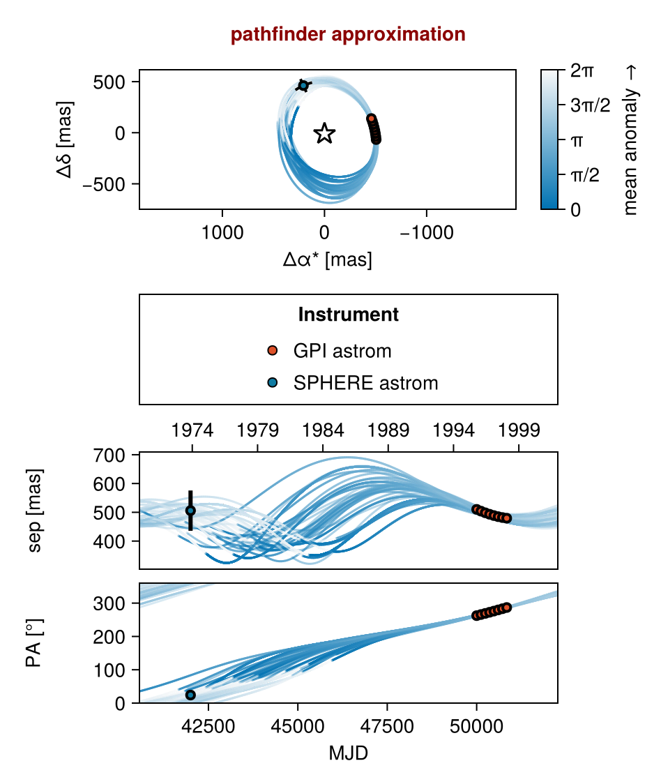
The starting points for sampling look reasonable!
The return value from initialize! is a "variational approximation". You can pass that chain to any function expecting a chain argument, like Octofitter.savechain or octocorner. It gives a very rough approximation of the posterior we expect.
Sampling
Now we are ready to draw samples from the posterior:
chain = octofit(model, iterations=1000)Chains MCMC chain (1000×35×1 Array{Float64, 3}):
Iterations = 1:1:1000
Number of chains = 1
Samples per chain = 1000
Wall duration = 5.36 seconds
Compute duration = 5.36 seconds
parameters = plx, b_M, b_a, b_e, b_i, b_ωx, b_ωy, b_Ωx, b_Ωy, b_θx, b_θy, b_ω, b_Ω, b_θ, b_plx, b_tp, b_GPI_astrom_jitter, b_GPI_astrom_northangle, b_GPI_astrom_platescale, b_SPHERE_astrom_jitter, b_SPHERE_astrom_northangle, b_SPHERE_astrom_platescale
internals = n_steps, is_accept, acceptance_rate, hamiltonian_energy, hamiltonian_energy_error, max_hamiltonian_energy_error, tree_depth, numerical_error, step_size, nom_step_size, is_adapt, loglike, logpost, tree_depth, numerical_error
Use `describe(chains)` for summary statistics and quantiles.
You will get an output that looks something like this with a progress bar that updates every second or so. You can reduce or completely silence the output by reducing the verbosity value down to 0 from a default of 2 (or get more info with verbosity=4).
Once complete, the chain object will hold the posterior samples. Displaying it prints out a summary table like the one shown above.
For a basic model like this with few epochs and well-specified uncertainties, sampling should take less than a minute on a typical laptop.
Sampling can take much longer when you have measurements with very small uncertainties (e.g. VLTI-GRAVITY).
Diagnostics
The first thing you should do with your results is check a few diagnostics to make sure the sampler converged as intended.
A few things to watch out for: check that you aren't getting many numerical errors (ratio_divergent_transitions). This likely indicates a problem with your model: either invalid values of one or more parameters are encountered (e.g. the prior on semi-major axis includes negative values) or that there is a region of very high curvature that is failing to sample properly. This latter issue can lead to a bias in your results.
One common mistake is to use a distribution like Normal(10,3) for semi-major axis. This left tail of this distribution includes negative values, and our orbit model is not defined for negative semi-major axes. A better choice is a truncated(Normal(10,3), lower=0.1) distribution (not including zero, since a=0 is not defined).
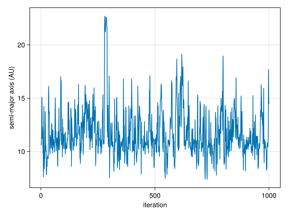
Next, you can make a trace plot of different variabes to visually inspect the chain:
using CairoMakie
lines(
    chain["b_a"][:],
    axis=(;
        xlabel="iteration",
        ylabel="semi-major axis (AU)"
    )
)
And an auto-correlation plot:
using StatsBase
using CairoMakie
lines(
    autocor(chain["b_e"][:], 1:500),
    axis=(;
        xlabel="lag",
        ylabel="autocorrelation",
    )
)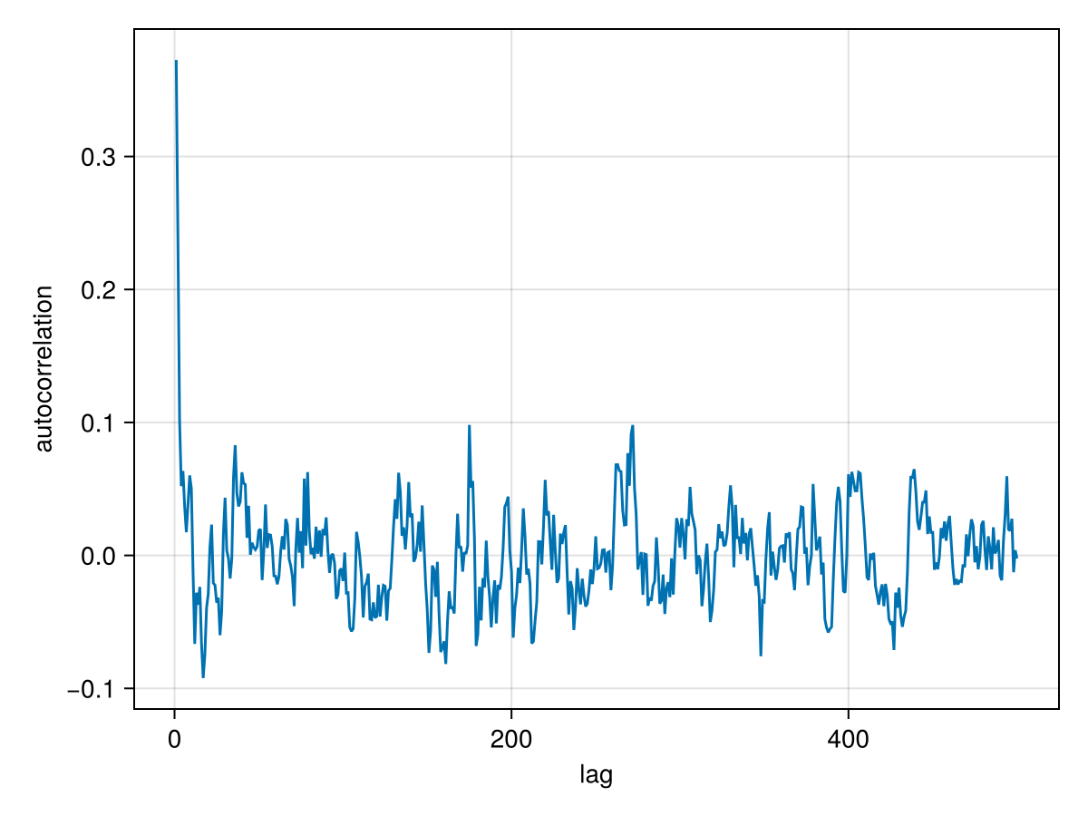
This plot shows that these samples are not correlated after only about 5 iterations. No thinning is necessary.
To confirm convergence, you may also examine the rhat column from chains. This diagnostic approaches 1 as the chains converge and should at the very least equal 1.0 to one significant digit (3 recommended).
Finaly, you might consider running multiple chains. Simply run octofit multiple times, and store the result in different variables. Then you can combine the chains using chainscat and run additional inter-chain convergence diagnostics:
using MCMCChains
chain1 = octofit(model)
chain2 = octofit(model)
chain3 = octofit(model)
merged_chains = chainscat(chain1, chain2, chain3)
gelmandiag(merged_chains)
Gelman, Rubin, and Brooks diagnostic
parameters psrf psrfci
Symbol Float64 Float64
plx 1.0002 1.0008
b_M 1.0029 1.0107
b_a 1.0040 1.0078
b_e 1.0002 1.0005
b_i 1.0110 1.0207
b_ωx 1.0058 1.0218
b_ωy 1.0013 1.0061
b_Ωx 1.0102 1.0375
b_Ωy 1.0087 1.0313
b_θx 1.0010 1.0033
b_θy 1.0004 1.0012
b_ω 1.0013 1.0037
b_Ω 1.0075 1.0257
b_θ 1.0014 1.0036
b_plx 1.0002 1.0008
⋮ ⋮ ⋮
7 rows omitted
This will check that the means and variances are similar between chains that were initialized at different starting points.
Analysis
As a first pass, let's plot a sample of orbits drawn from the posterior. The function octoplot is a conveninient way to generate a 9-panel plot of velocities and position:
using CairoMakie
octoplot(model,merged_chains)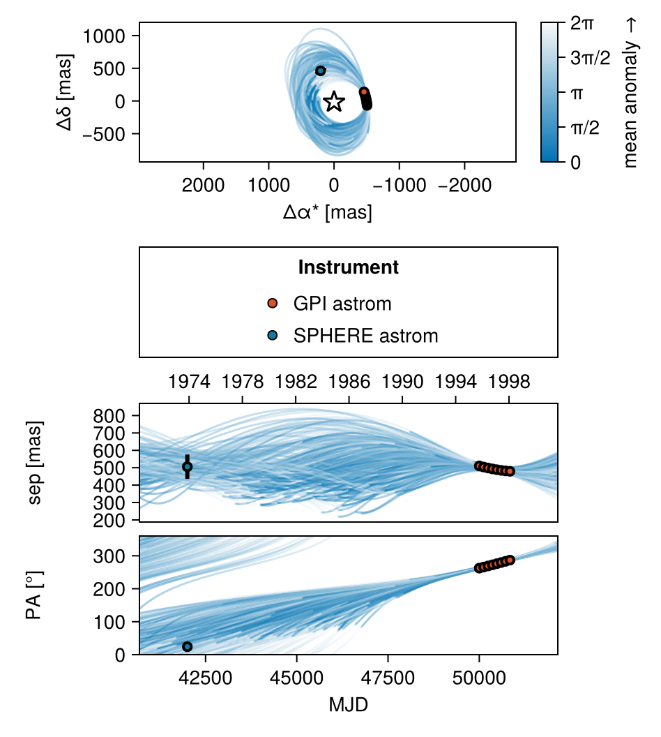
This function draws orbits from the posterior and displays them in a plot. Any astrometry points are overplotted.
You can control what panels are displayed, the time range, colourscheme, etc. See the documentation on octoplot for more details.
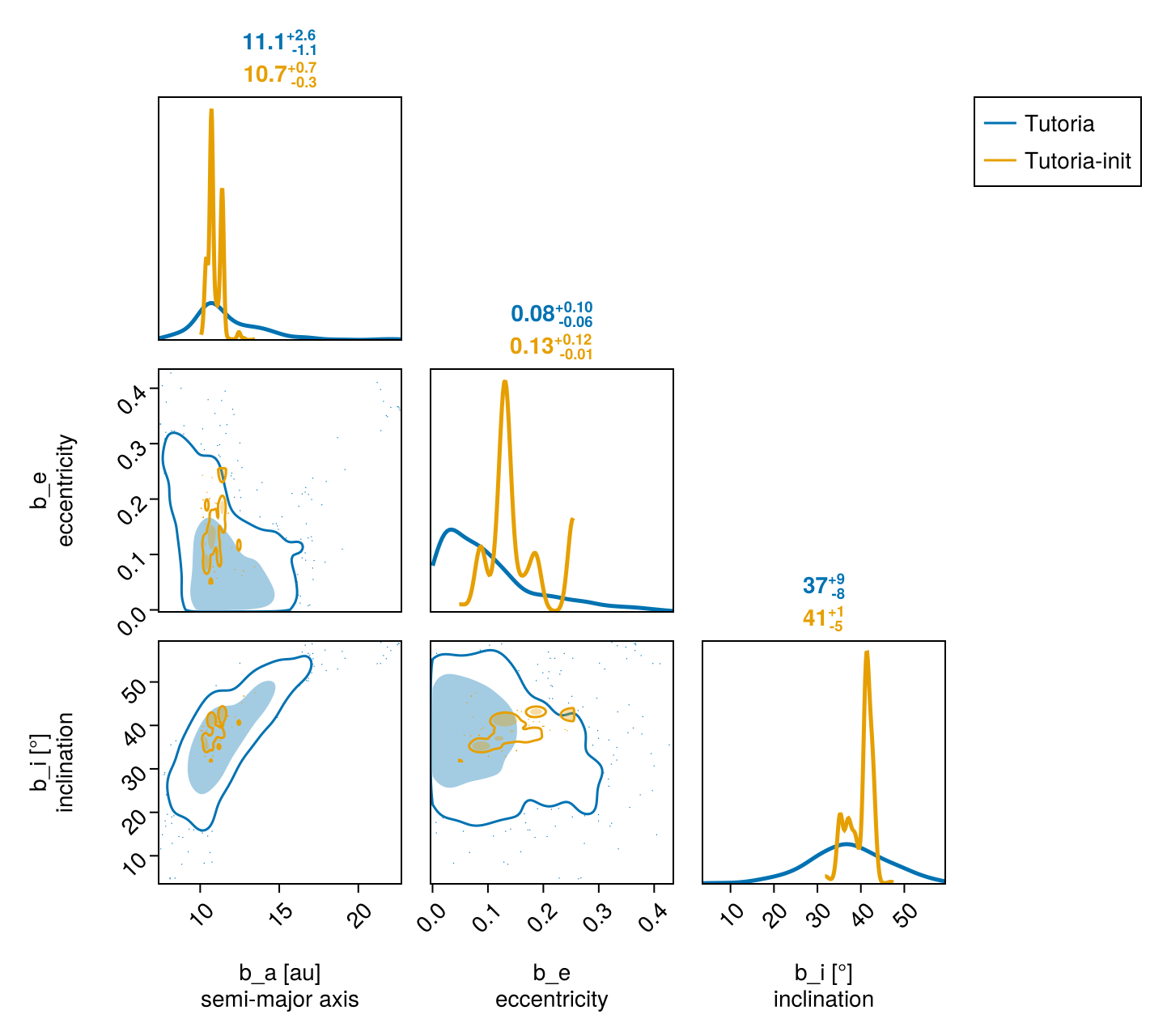
Pair Plot
A very useful visualization of our results is a pair-plot, or corner plot. We can use the octocorner function and our PairPlots.jl package for this purpose:
using CairoMakie
using PairPlots
octocorner(model, merged_chains, small=true)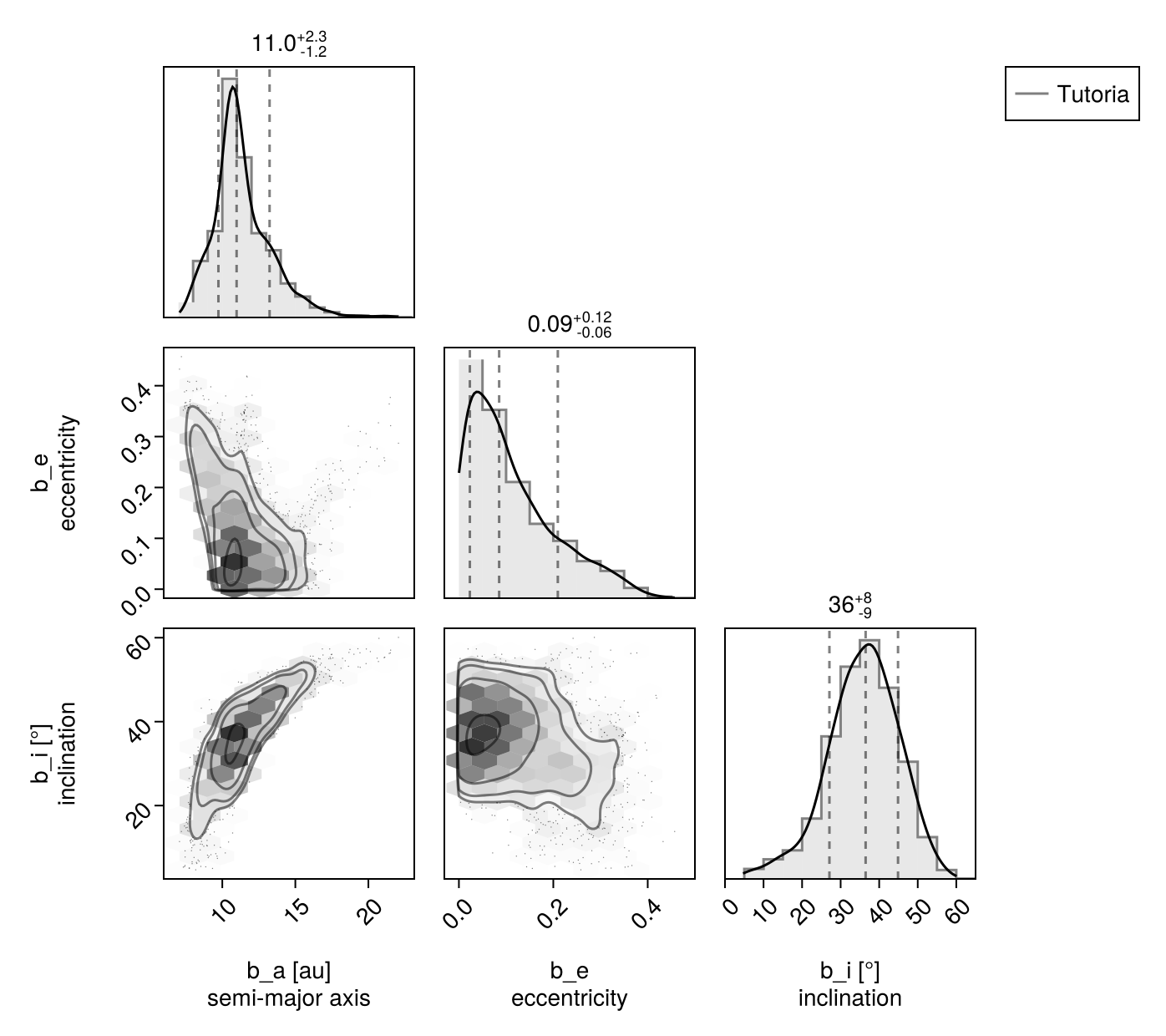
Remove small=true to display all variables.
In this case, the sampler was able to resolve the complicated degeneracies between eccentricity, the longitude of the ascending node, and argument of periapsis.
Saving your chain
Variables can be retrieved from the chains using the following sytnax: sma_planet_b = chain["b_a",:,:]. The first index is a string or symbol giving the name of the variable in the model. Planet variables are prepended by the name of the planet and an underscore.
You can save your chain in FITS table format by running:
Octofitter.savechain("mychain.fits", chain)You can load it back via:
chain = Octofitter.loadchain("mychain.fits")Saving your model
You may choose to save your model so that you can reload it later to make plots, etc:
using Serialization
serialize("model1.jls", model)
Which can then be loaded at a later time using:
using Serialization
using Octofitter # must include all the same imports as your original script
model = deserialize("model1.jls")Serialized models are only loadable/restorable on the same computer, version of Octofitter, and version of Julia. They are not intended for long-term archiving. For reproducibility, make sure to keep your original model definition script.
Comparing chains
We can compare two different chains by passing them both to octocorner. Let's compare the init_chain with the full results from octofit:
octocorner(model, chain, init_chain, small=true)