Prior Predictive Checks

The prior predictive distributin of a Bayesian model what you get by sampling parameters directly from the priors and calculating where the model would place the data. For example, if sampling from relative astrometry, the prior predictive model is the distribution of (simulated) astrometry points corresponding to orbits drawn from the prior. For radial velocity data, these would be simulated RV points based on an RV curve drawn from the priors.

To generate a prior predictive distribution, one first needs to create a model. We will use the model and sample data from the Fit Astrometry tutorial:

using Octofitter
using CairoMakie
using PairPlots
using Distributions

astrom_like = PlanetRelAstromLikelihood(Table(;
    epoch= [50000,50120,50240,50360,50480,50600,50720,50840,],
    ra = [-505.764,-502.57,-498.209,-492.678,-485.977,-478.11,-469.08,-458.896,],
    dec = [-66.9298,-37.4722,-7.92755,21.6356, 51.1472, 80.5359, 109.729, 138.651,],
    σ_ra = fill(10.0, 8),
    σ_dec = fill(10.0, 8),
    cor = fill(0.0, 8)
))
@planet b Visual{KepOrbit} begin
    a ~ truncated(Normal(10, 4), lower=0, upper=100)
    e ~ Uniform(0.0, 0.5)
    i ~ Sine()
    ω ~ UniformCircular()
    Ω ~ UniformCircular()
    θ ~ UniformCircular()
    tp = θ_at_epoch_to_tperi(system,b,50420)  # reference epoch for θ. Choose an MJD date near your data.
end astrom_like
@system Tutoria begin
    M ~ truncated(Normal(1.2, 0.1), lower=0)
    plx ~ truncated(Normal(50.0, 0.02), lower=0)
end b

We can now draw one sample from the prior:

prior_draw_system = generate_from_params(Tutoria)
prior_draw_astrometry = prior_draw_system.planets.b.observations[4]

PlanetRelAstromLikelihood Table with 5 columns and 8 rows:
     epoch  ra        dec       σ_ra  σ_dec
   ┌───────────────────────────────────────
 1 │ 50000  -65.5338  78.7773   10.0  10.0
 2 │ 50120  -39.9935  62.6296   10.0  10.0
 3 │ 50240  -14.3355  46.298    10.0  10.0
 4 │ 50360  11.3639   29.8331   10.0  10.0
 5 │ 50480  37.0316   13.284    10.0  10.0
 6 │ 50600  62.5972   -3.30198  10.0  10.0
 7 │ 50720  87.9934   -19.8791  10.0  10.0
 8 │ 50840  113.155   -36.4035  10.0  10.0

And plot the generated astrometry:

Makie.scatter(prior_draw_astrometry.table.ra, prior_draw_astrometry.table.dec,color=:black, axis=(;autolimitaspect=1,xreversed=true))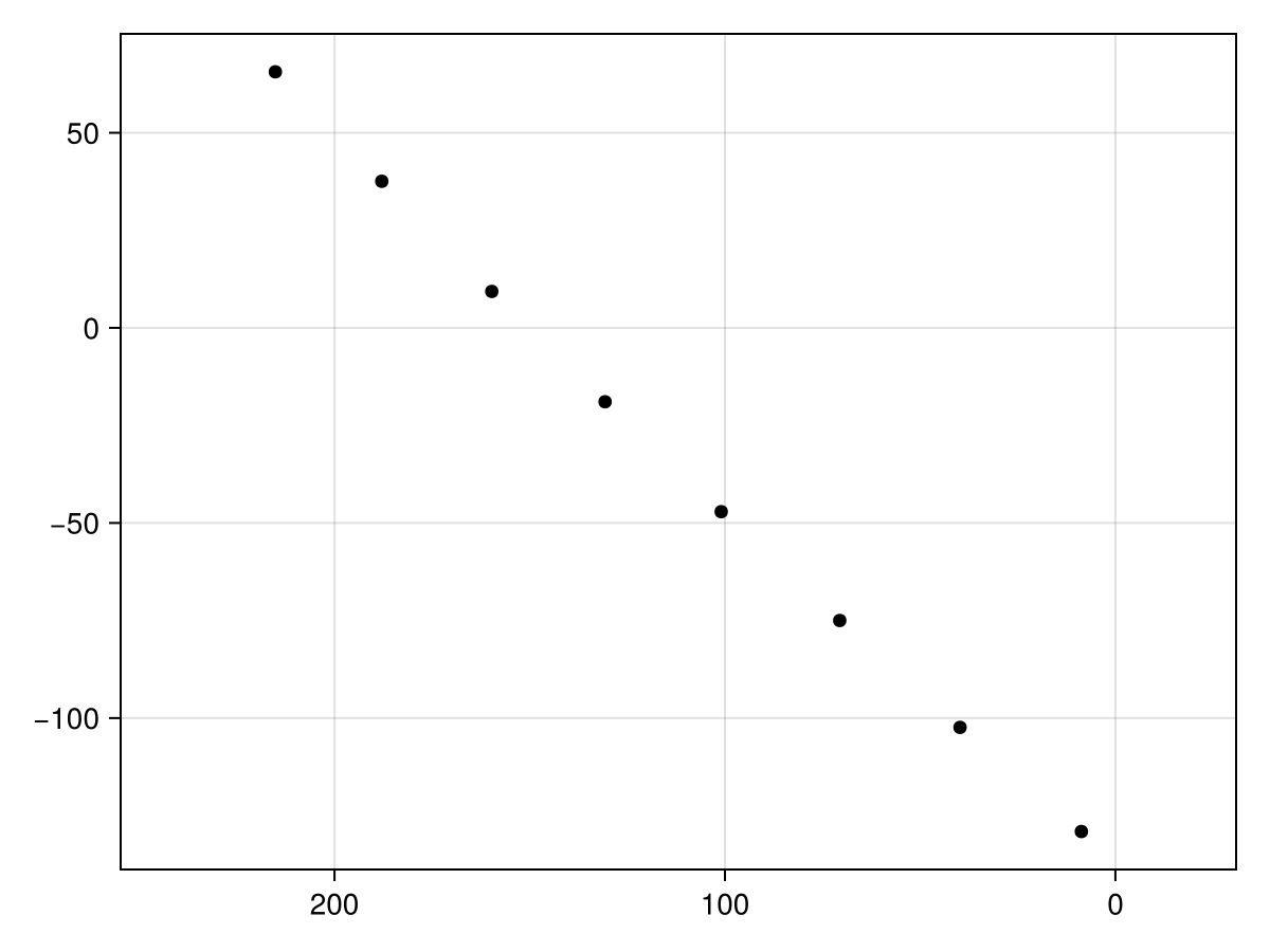

We can repeat this many times to get a feel for our chosen priors in the domain of our data:

using Random
Random.seed!(1)


fig = Figure()
ax = Axis(
    fig[1,1], xlabel="ra offset [mas]", ylabel="dec offset [mas]",
    xreversed=true,
    aspect=1
)
for i in 1:50
    prior_draw_system = generate_from_params(Tutoria)
    prior_draw_astrometry = prior_draw_system.planets.b.observations[4]
    Makie.scatter!(
        ax,
        prior_draw_astrometry.table.ra,
        prior_draw_astrometry.table.dec,
        color=Makie.cgrad(:turbo)[i/50],
    )
end

fig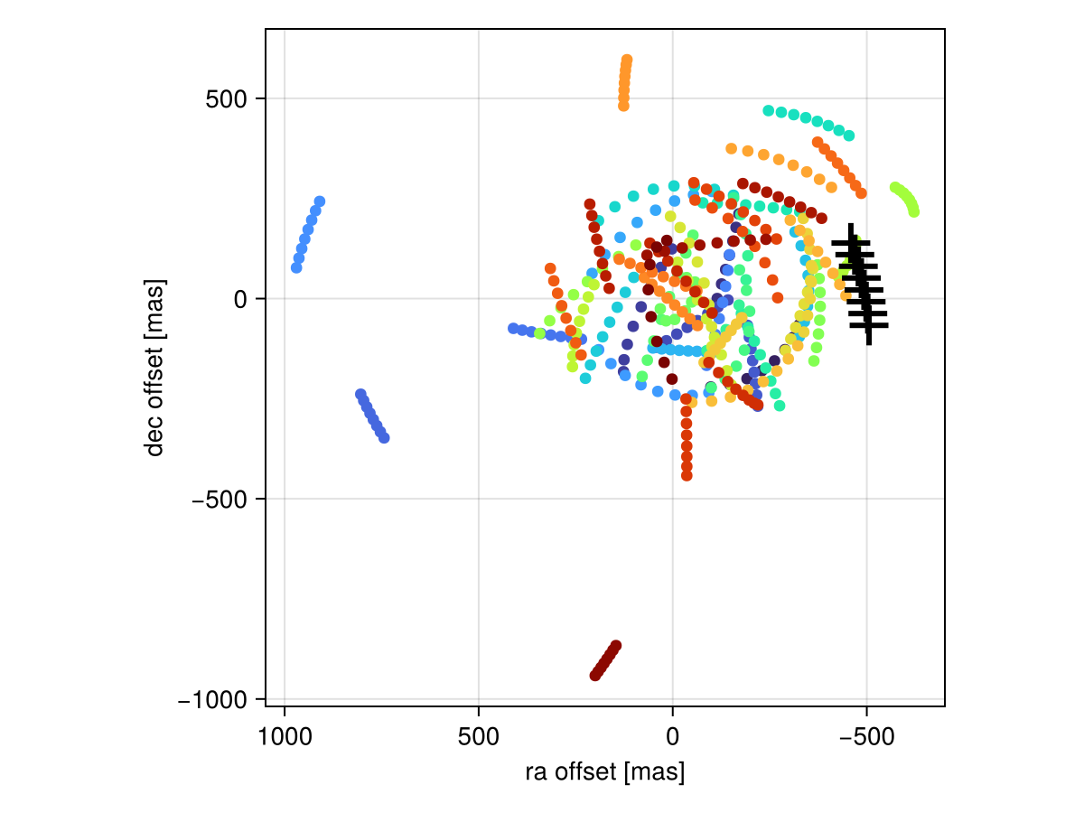

The heavy black crosses are our actual data, while the colored ones are simulations drawn from our priors. Notice that our real data lies at a greater separation than most draws from the prior? That might mean the priors could be tweaked.