Multi-Planet RV Fits
This tutorial shows how to perform a multi-planet RV fit, and compare the bayesian evidence between the two models.
octofit_pigeons and Pigeons.stepping_stone are how Octofitter computes a log Bayesian evidence, and octofit_pigeons's methods live in a package extension — so pkg> add Pigeons and using Pigeons are required before the sampling blocks on this page, or they fail with a MethodError. If you only want the posteriors and not the evidence, octofit(model) (HMC) samples these models fine.
using Octofitter
using OctofitterRadialVelocity
using CairoMakie
using PairPlots
using Distributions
using PlanetOrbits
To begin, we create simulated data. We imagine that we have two different instruments.
A synthetic system is a real PlanetOrbits.System: the star and both planets have masses, and the hierarchy says what orbits what. Solving it once gives the star's reflex velocity directly, with no need to sum radvel over each planet by hand.
using Random
Random.seed!(1)

star = PlanetOrbits.Body(mass=1.0,     name=:A)   # M⊙
p_b  = PlanetOrbits.Body(mass=0.25e-3, name=:b)   # M⊙
p_c  = PlanetOrbits.Body(mass=1.0e-3,  name=:c)   # M⊙

truth = PlanetOrbits.System(
    (star, p_b, p_c),
    (
        PlanetOrbits.Orbit(p_b, about=star;        a=1.0, e=0.05, ω=1pi/4, i=pi/2, Ω=0.0, tp=58800),
        PlanetOrbits.Orbit(p_c, about=(star, p_b); a=5.0, e=0.40, ω=1pi/4, i=pi/2, Ω=0.0, tp=59800),
    )
)

"The star's reflex velocity against the system barycentre, in m/s."
function reflex_rv(epochs)
    traj = orbitsolve(truth, epochs)
    return [radvel(traj[k], :A, barycentre(truth)) for k in eachindex(epochs)]
end

epochs1 = (58400:150:69400) .+ 10 .* randn.()
rv1 = reflex_rv(epochs1)
rvlike1 = MarginalizedRVObs(
    Table(epoch=epochs1, rv=rv1 .+ 4 .* randn.(), σ_rv=[4 * abs(randn()) + 1 for _ in eachindex(epochs1)]);
    target=:A, ref=Barycentre,
    name="DATA 1",
    variables=@variables begin
        jitter ~ LogUniform(0.1, 100) # m/s
    end
)

epochs2 = (65400:100:71400) .+ 10 .* randn.()
rv2 = reflex_rv(epochs2)
rvlike2 = MarginalizedRVObs(
    Table(epoch=epochs2, rv=rv2 .+ 2 .* randn.() .+ 7, σ_rv=[2 * abs(randn()) + 1 for _ in eachindex(epochs2)]);
    target=:A, ref=Barycentre,
    name="DATA 2",
    variables=@variables begin
        jitter ~ LogUniform(0.1, 100) # m/s
    end
)

fig = Figure()
ax = Axis(
    fig[1,1],
    xlabel="epoch [mjd]",
    ylabel="rv [m/s]"
)
Makie.scatter!(ax, rvlike1.table.epoch, rvlike1.table.rv)
Makie.errorbars!(ax, rvlike1.table.epoch, rvlike1.table.rv, rvlike1.table.σ_rv)
Makie.scatter!(ax, rvlike2.table.epoch, rvlike2.table.rv)
Makie.errorbars!(ax, rvlike2.table.epoch, rvlike2.table.rv, rvlike2.table.σ_rv)
fig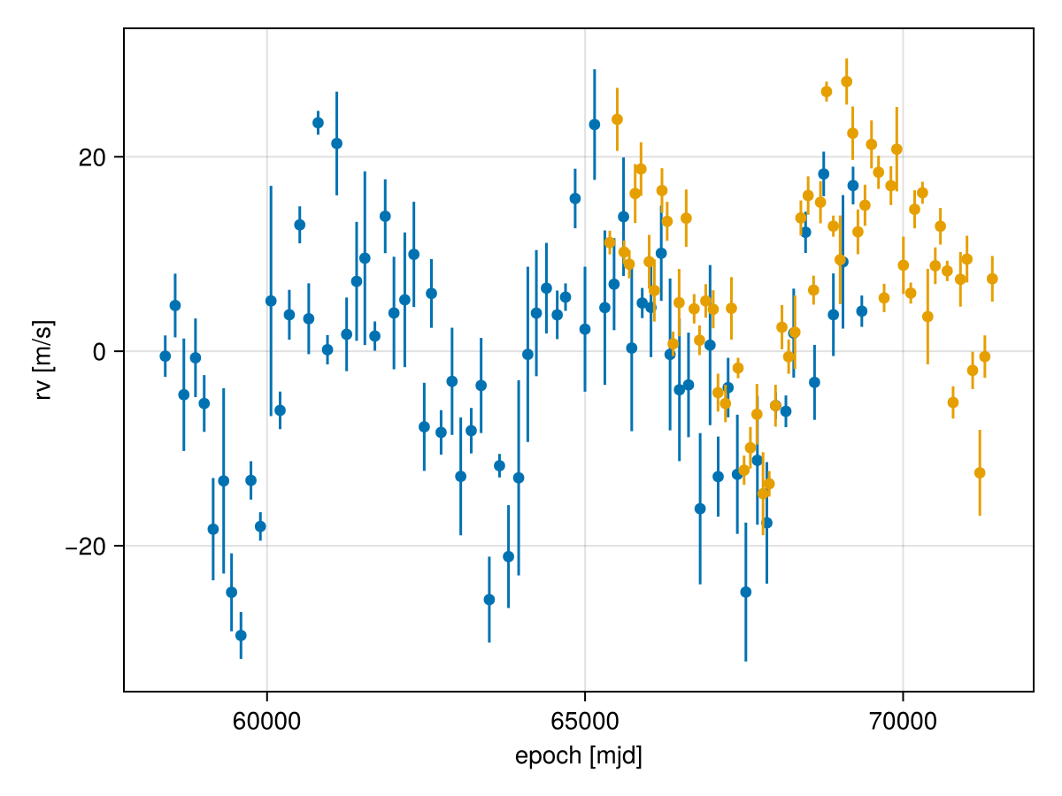
MarginalizedRVObs analytically marginalizes out each instrument's radial velocity zero point. It requires target= (with ref= defaulting to Barycentre), and it errors if you declare an offset variable.
Two Planet Model
We will set up a Jacobi chain—that means the outer planet will orbit the barycentre of the star and inner planet together, and see both of their masses as the "central body". If you use the N-Body integrator, this is just a convention about what the orbit parameters refer to. If you use the default plain Kepler solver, it will make a big difference if the inner companion mass is not $\ll$ the host mass.
Concretely: - about=A — the planet orbits the star alone (astrocentric). - about=(A, b) — the planet orbits the barycentre of the star and the inner planet (Jacobi), so its orbit's mass is M_A + M_b + M_c.
Below, b is the inner planet and c the outer one, so c is placed about (A, b).
A = Body(
    name="A",
    variables=@variables begin
        mass = 1.0                  # M⊙
    end
)

planet_b = Body(
    name="b",
    about=A,
    variables=@variables begin
        # RV-only: the inclination and node are unconstrained, so fix them.
        i = pi/2
        Ω = 0.0
        e ~ Uniform(0,0.999999)
        ω ~ Uniform(0,2pi)
        mass ~ Uniform(0, 10mjup)   # M⊙

        P ~ Uniform(0, 100year2day_julian)
        τ ~ Uniform(0,1.0)
        tp = τ*P + 58400
    end
)

planet_c = Body(
    name="c",
    about=(A, planet_b),            # Jacobi: c orbits the A+b barycentre
    variables=@variables begin
        i = pi/2
        Ω = 0.0
        e ~ Uniform(0,0.999999)
        ω ~ Uniform(0,2pi)
        mass ~ Uniform(0, 10mjup)   # M⊙

        P ~ Uniform(0, 100year2day_julian)
        τ ~ Uniform(0,1.0)
        tp = τ*P + 58400
    end
)

sim_2p = System(
    name="sim_2p",
    bodies=[A, planet_b, planet_c],
    observations=[rvlike1, rvlike2],
)

model_2p = Octofitter.LogDensityModel(sim_2p)
LogDensityModel for System sim_2p of dimension 12 and 135 epochs with fields .ℓπcallback and .∇ℓπcallback
Sample from the posterior
using Pigeons
results_2p, pt_2p = octofit_pigeons(model_2p, n_rounds=10)
(chain = MCMC chain (1024×23×1 Array{Float64, 3}), pt = PT(checkpoint = false, ...))If you have an expensive model – say, lots of companions, or a thousand RV data points – consider using multiple cores or submiting to a cluster with MPI. Run:
results_2p, pt_2p = octofit_pigeons(model_2p, n_rounds=10, cores=8)Set cores to the number of CPU cores you want to use. Each run spends a minute or two starting workers before sampling begins, so this pays off for longer fits. See octofit_pigeons.
Now plot the posterior compared to the data for one draw:
rvplot(model_2p, results_2p)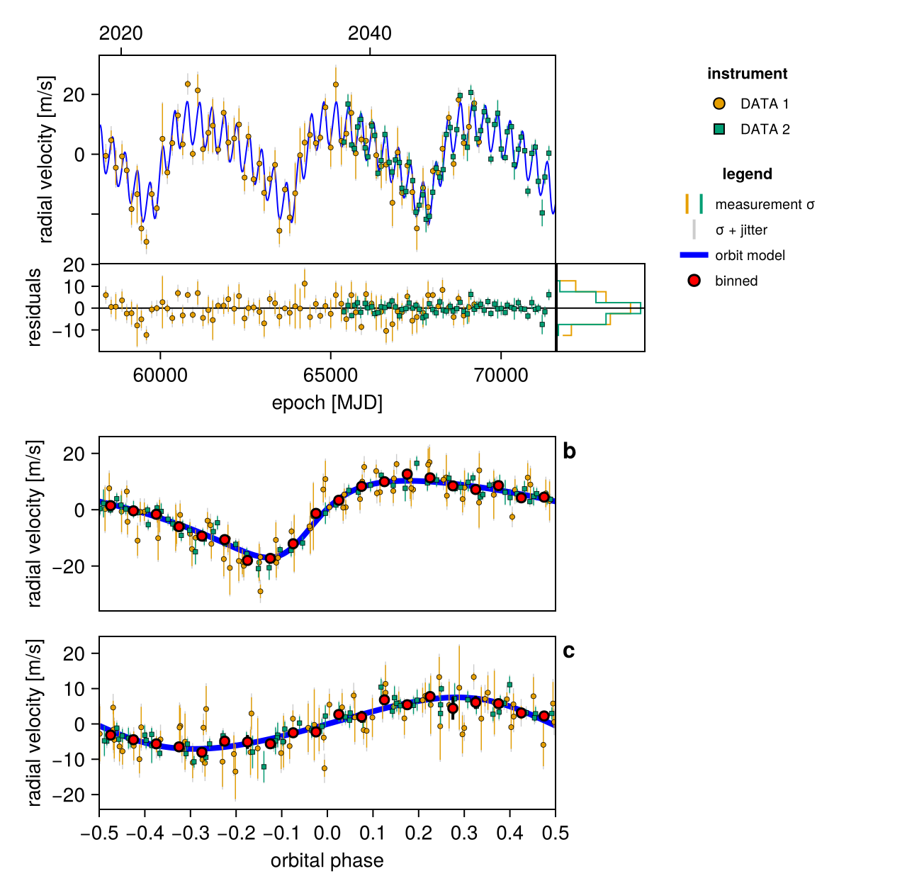
...and a sample of many draws:
octoplot(model_2p, results_2p)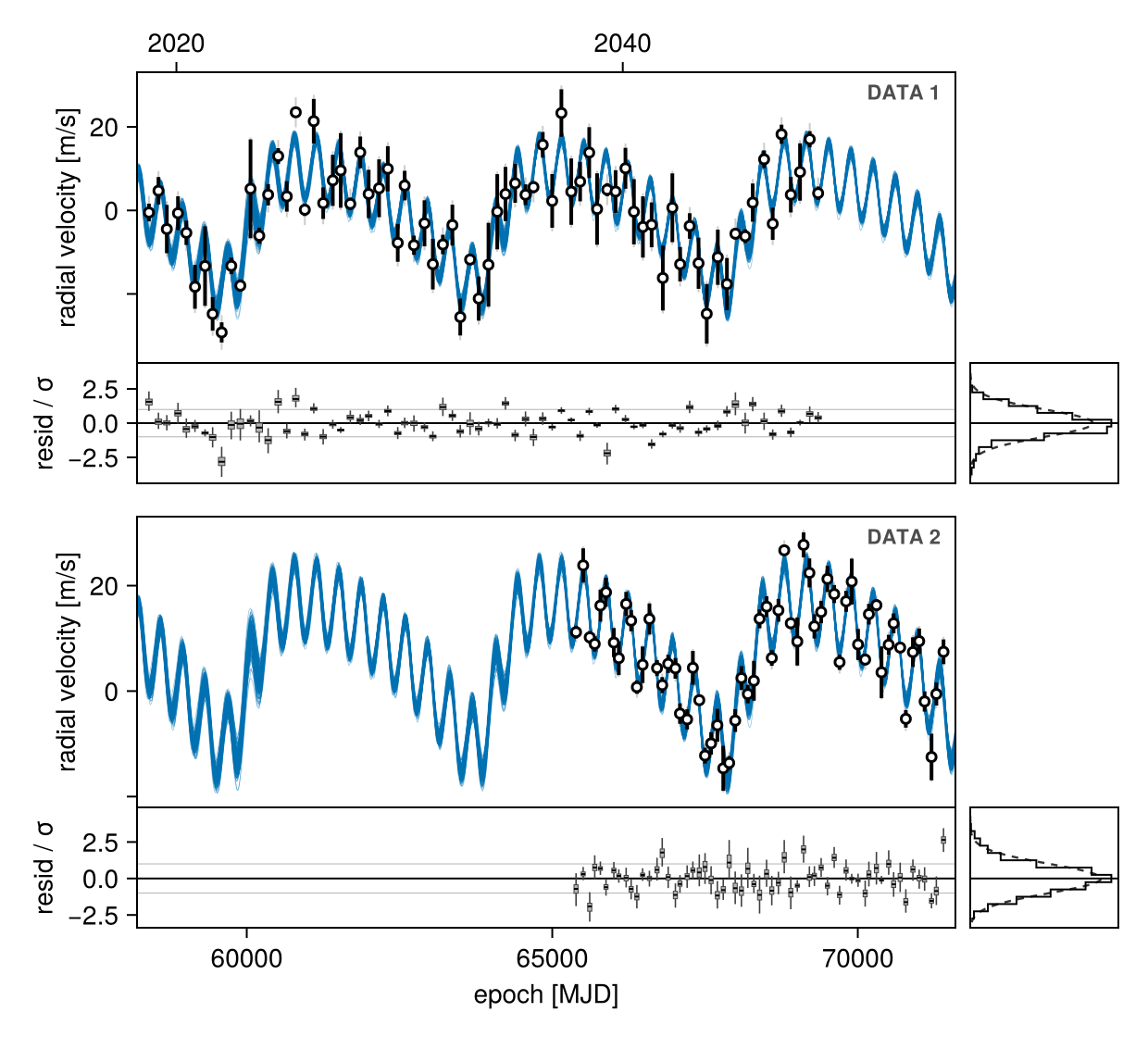
One Planet Model
We now create a new system object that only includes one planet (we dropped c, in this case). planet_b can be reused as-is:
sim_1p = System(
    name="sim_1p",
    bodies=[A, planet_b],
    observations=[rvlike1, rvlike2],
)

model_1p = Octofitter.LogDensityModel(sim_1p)
LogDensityModel for System sim_1p of dimension 7 and 135 epochs with fields .ℓπcallback and .∇ℓπcallback
Sample from the posterior
using Pigeons
results_1p, pt_1p = octofit_pigeons(model_1p, n_rounds=10)
(chain = MCMC chain (1024×15×1 Array{Float64, 3}), pt = PT(checkpoint = false, ...))Plot RV curve, phase folded curve, and binned residuals.
For one draw at a time:
rvplot(model_1p, results_1p)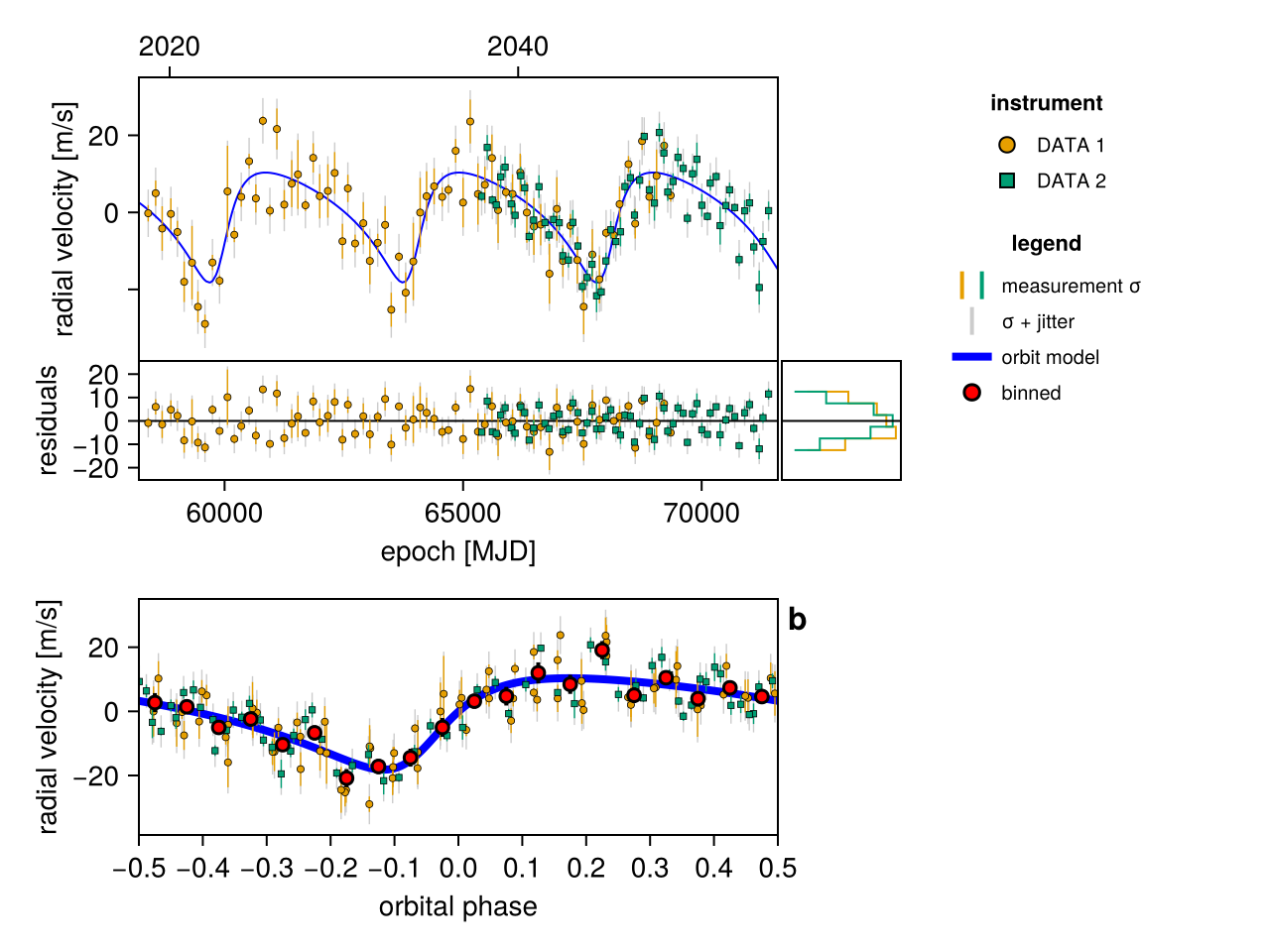
For a sample of draws:
octoplot(model_1p, results_1p)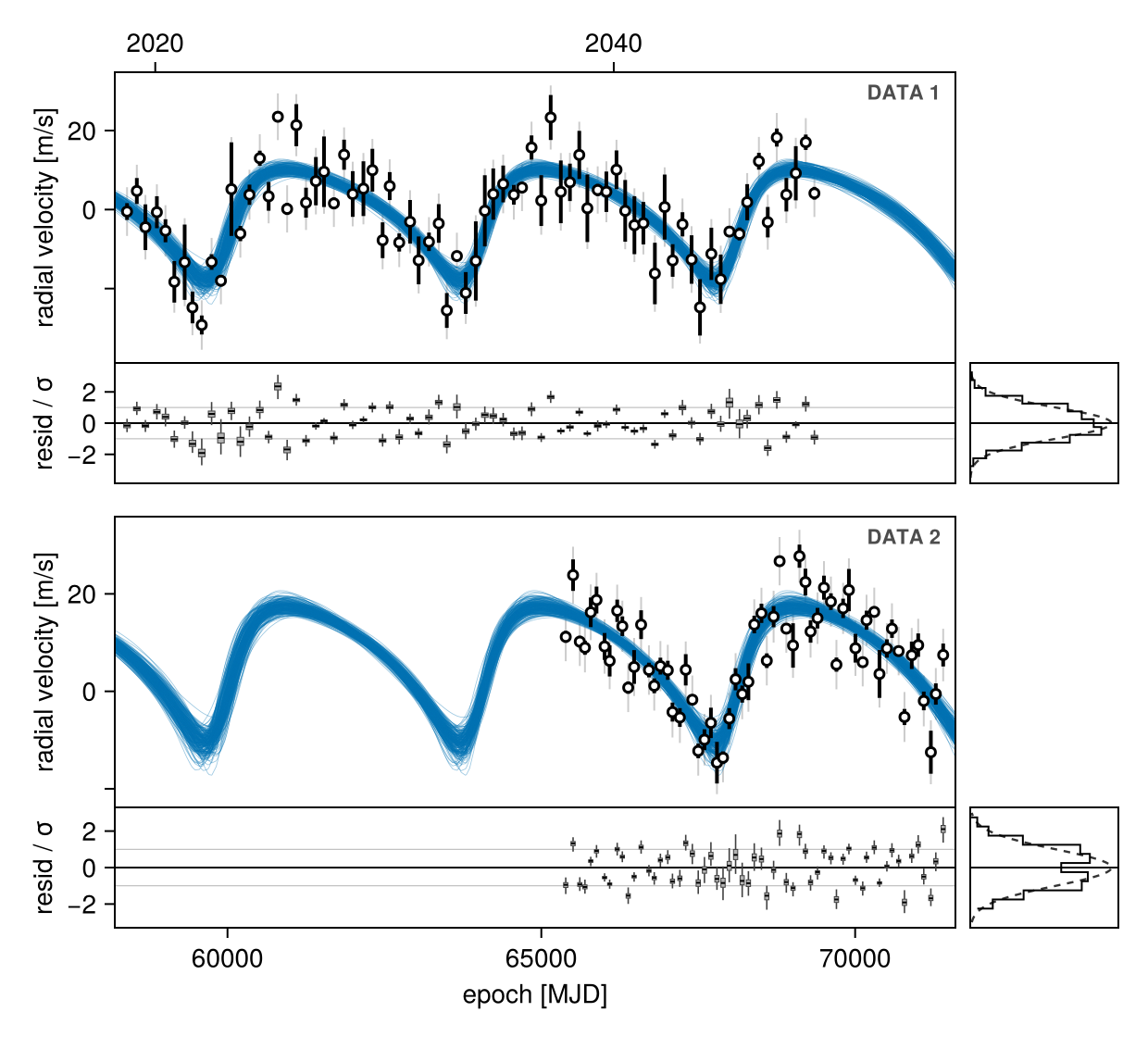
Model Comparison: Bayesian Evidence
Octofitter with Pigeons directly calculates the (natural) log Bayesian evidence using the "stepping stone" method. This should be more reliable than even nested sampling, and certainly more reliable than approximate methods like the BIC/WAIC etc.
Z1 = stepping_stone(pt_1p)
Z2 = stepping_stone(pt_2p)

ln_BF₁₀ = Z2-Z150.13095136813092Here is a standard guideline you can use to interpret the evidence:
| Log Bayes Factor ln(BF₁₀) | Interpretation |
|---|---|
| > 3.00 | Extreme evidence for $H_A$ |
| 1.61 - 3.00 | Very strong evidence for $H_A$ |
| 1.10 - 1.61 | Strong evidence for $H_A$ |
| 0.69 - 1.10 | Moderate evidence for $H_A$ |
| 0 - 0.69 | Anecdotal evidence for $H_A$ |
| 0 | No evidence |
| -0.69 - 0 | Anecdotal evidence for $H_B$ |
| -1.10 - -0.69 | Moderate evidence for $H_B$ |
| -1.61 - -1.10 | Strong evidence for $H_B$ |
| -3.00 - -1.61 | Very strong evidence for $H_B$ |
| < -3.00 | Extreme evidence for $H_B$ |
As you can see, the evidence for there being two planets is "extreme" in this case. Try adjusting the masses of the two planets and see how this changes!
Parameterizations
When using the evidence for model comparisons, a model with more specific priors will have more evidence than an quivalent model with broad priors.
In our two planet model above, we made two exactly equivalent planets. If you inspect the chains, you may notice that the two planets often flip back and forth – sometimes b has the longer period, and sometimes c does.
For example, here is a histogram of the period of planet b:
hist(vec(results_2p[:b_P]) ./ year2day_julian, bins=100)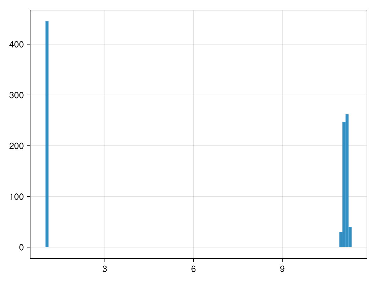
We can refine the two planet model a bit by adjusting the priors such that planet c always has a longer period than planet b.
This will make analysis a little more straightforward, but it will also increase the evidence of this model by approximately halving the prior volume—thus making a more specific prediction.
There are several ways we could do this. Here, we add a "nominal period" variable and reparameterize the two planets as ratios of this nominal period.
Octofitter also ships an OrbitOrderPrior, which enforces a_b < a_c directly by rejecting draws where the ordering is violated.
planet_b_v2 = Body(
    name="b",
    about=A,
    variables=@variables begin
        i = pi/2
        Ω = 0.0
        e ~ Uniform(0,0.999999)
        ω ~ Uniform(0,2pi)
        mass ~ Uniform(0, 10mjup)   # M⊙

        P = system.P_nom * system.P_ratio_b
        τ ~ Uniform(0,1.0)
        tp = τ*P + 58400
    end
)

planet_c_v2 = Body(
    name="c",
    about=(A, planet_b_v2),
    variables=@variables begin
        i = pi/2
        Ω = 0.0
        e ~ Uniform(0,0.999999)
        ω ~ Uniform(0,2pi)
        mass ~ Uniform(0, 10mjup)   # M⊙

        P = system.P_nom * system.P_ratio_c
        τ ~ Uniform(0,1.0)
        tp = τ*P + 58400
    end
)


sim_2p_v2 = System(
    name="sim_2p_v2",
    bodies=[A, planet_b_v2, planet_c_v2],
    observations=[rvlike1, rvlike2],
    variables=@variables begin
        P_nom ~ Uniform(0, 100year2day_julian)
        P_ratio_b ~ Uniform(0, 0.5)
        P_ratio_c ~ Uniform(0.5, 1)
    end
)

model_2p_v2 = Octofitter.LogDensityModel(sim_2p_v2)
LogDensityModel for System sim_2p_v2 of dimension 13 and 135 epochs with fields .ℓπcallback and .∇ℓπcallback
Sample from the posterior
using Pigeons
results_2p_v2, pt_2p_v2 = octofit_pigeons(model_2p_v2, n_rounds=10)
The planet with the wider orbit is now consistently plotted in the same panel (meaning that planet b and c are no longer trading back and forth):
octoplot(model_2p_v2, results_2p_v2)If we look again at the log-evidence, we see that this parameterization (Z3) is even more favoured. This is because this small change in parameterization makes considerably
Z1 = stepping_stone(pt_1p)
Z2 = stepping_stone(pt_2p)
Z3 = stepping_stone(pt_2p_v2)

Z1, Z2, Z3
All the plots above overlay many posterior draws. To inspect one draw at a time — for example the maximum a-posteriori sample — slice the chain:
i_map = argmax(vec(results_2p_v2[:logpost])) # find index of highest posteriori sample *in the chain*
rvplot(model_2p_v2, results_2p_v2, i_map) # plot this specific draw index
You should probably look at that plot for a good number of different draws, not just one.
Analyzing Period Ratios
For studies of mean motion resonances, it's useful to examine the posterior distribution of the period ratio between planets. You can compute this directly from the chains:
# Extract period samples for each planet
P_b_samples = vec(results_2p_v2[:b_P])
P_c_samples = vec(results_2p_v2[:c_P])

# Compute period ratio (outer/inner)
period_ratios = P_c_samples ./ P_b_samples

# Plot histogram
fig = Figure()
ax = Axis(fig[1,1], xlabel="Period Ratio (Pc/Pb)", ylabel="Density")
hist!(ax, period_ratios, bins=50, normalization=:pdf)
fig
This approach works for any multi-planet model and can help identify potential mean motion resonances.
Note about the evidence ratio
The pigeons method returns the log evidence ratio. If the priors are properly normalized, this is equal to the log evidence.
In other cases (e.g. if using ObsPriorONeil2019 or UniformCircular) you may need to calculate the log_Z0 term yourself. This can be done as follows:
prior_model = Octofitter.LogDensityModel(Octofitter.prior_only_model(model_1p.system, exclude_all=true))
_, pt_prior = octofit_pigeons(prior_model, n_rounds=10) # should be very quick!
log_Z0 = stepping_stone(pt_prior)0.0041204622443595795Subtract this from the stepping stone value to get the true evidence:
log_Z1_over_Z0 = stepping_stone(pt_1p)
log_Z1 = log_Z1_over_Z0 - log_Z0
-461.7635148167758