Fit Proper Motion Anomaly
Octofitter.jl supports fitting orbit models to astrometric motion in the form of GAIA-Hipparcos proper motion anomaly (HGCA; https://arxiv.org/abs/2105.11662). These data points are calculated by finding the difference between a long term proper motion of a star between the Hipparcos and GAIA catalogs, and their proper motion calculated within the windows of each catalog. This gives four data points that can constrain the dynamical mass & orbits of planetary companions (assuming we subtract out the net trend).
If your star of interest is in the HGCA, all you need is it's GAIA DR3 ID number. You can find this number by searching for your target on SIMBAD.
For this tutorial, we will examine the star and companion HD 91312 A & B discovered by SCExAO. We will use their published astrometry and proper motion anomaly extracted from the HGCA.
We will also perform a model comparison: we will fit the same model to four different subsets of data to see how each dataset are impacting the final constraints. This is an important consistency check, especially with proper motion / absolute astrometry data which be susceptible to systematic errors.
The first step is to find the GAIA source ID for your object. For HD 91312, SIMBAD tells us the GAIA DR3 ID is 756291174721509376.
Fitting Astrometric Motion Only
Initial setup:
using Octofitter, Distributions, RandomWe begin by finding orbits that are consistent with the astrometric motion. Later, we will add in relative astrometry to the fit from direct imaging to further constrain the planet's orbit and mass.
Compared to previous tutorials, we will now have to add a few additional variables to our model. The first is a prior on the mass of the companion, called mass. The units used on this variable are Jupiter masses, in contrast to M, the primary's mass, in solar masses. A reasonable uninformative prior for mass is Uniform(0,1000) or LogUniform(1,1000) depending on the situation.
For this model, we also want to place a prior on the host star mass rather than system total mass. For exoplanets there is litte difference between these two values, but in this example we have a reasonably informative prior on the host mass, and know from the paper that the companion is has a non-neglible effect on the total system mass.
To make this parameterization change, we specify priors on both masses in the @system block, and connect it to the planet.
Retrieving the HGCA
To start, we retrieve the HGCA data for this object.
hgca_obs = HGCAObs(
    gaia_id=3937211745905473024,
    variables=@variables begin
        # Optional: flux ratio for luminous companions, one entry per companion
        # fluxratio ~ Product([Uniform(0, 1), Uniform(0, 1), ])  # uncomment if needed for unresolved companions
    end
)
You can optionally provide flux ratio priors in the variables block to represent the flux ratio of the companions to the host, if you don't want to approximate it as zero. This is to handle luminous companions that are unresolved by gaia.
If you're in a hurry, and you're study orbits with periods much longer than the mission durations of Gaia or Hipparcos (>> 4 years) then you might consider using a faster approximation that the Gaia and Hipparcos measurements were instantaneous. You can do so as follows:
hgca_obs = HGCAInstantaneousObs(gaia_id=756291174721509376, N_ave=1)HGCAInstantaneousObs Table with 3 columns and 4 rows:
epoch meas inst
┌────────────────────
1 │ 48345.7 ra hip
2 │ 48500.8 dec hip
3 │ 57423.6 ra gaia
4 │ 57503.4 dec gaiaN_ave is an optional argument to control over how many epochs the measurements are approximated, e.g. N_ave=10 implies that the position and proper motion was measured instantaneously 10 times over each mission and averaged.
Planet Model
planet_b = Planet(
    name="b",
    basis=Visual{KepOrbit},
    variables=@variables begin
        P ~ LogUniform(1/365.25, 10000)# Period in Julian years (1 day to 10000yrs)
        # Now convert to the units expected by Kepler's third law
        # The conversion factor accounts for the IAU definitions
        P_for_kepler = P * Octofitter.PlanetOrbits.year2day_julian / Octofitter.PlanetOrbits.kepler_year_to_julian_day_conversion_factor
        q ~ LogUniform(1e-5, 1)
        mass = q * system.M_pri / Octofitter.mjup2msol
        e ~ Uniform(0, 0.9)  # Eccentricity
        ω ~ Uniform(0, 2pi)  # Argument of periastron
        i ~ Sine()
        Ω ~ Uniform(0, 2pi)
        τ ~ Uniform(0.0, 1.0)  # Fraction of period past periastron
        M = system.M_pri + mass * Octofitter.mjup2msol
        # Now apply Kepler's third law: a^3 = P^2 * M
        # where P is in "Keplerian years", a in AU, M in solar masses
        a = cbrt(P_for_kepler^2 * M)
        tp = τ * P * 365.25 + 57388.5  # Time of periastron [MJD]
    end
)
Planet b
Derived:
P_for_kepler = (P * Octofitter.PlanetOrbits.year2day_julian) / Octofitter.PlanetOrbits.kepler_year_to_julian_day_conversion_factor
mass = (q * system.M_pri) / Octofitter.mjup2msol
M = system.M_pri + mass * Octofitter.mjup2msol
a = cbrt(P_for_kepler ^ 2 * M)
tp = τ * P * 365.25 + 57388.5
Priors:
P ~ Distributions.LogUniform{Float64}(a=0.0027378507871321013, b=10000.0)
q ~ Distributions.LogUniform{Float64}(a=1.0e-5, b=1.0)
e ~ Distributions.Uniform{Float64}(a=0.0, b=0.9)
ω ~ Distributions.Uniform{Float64}(a=0.0, b=6.283185307179586)
i ~ Sine()
Ω ~ Distributions.Uniform{Float64}(a=0.0, b=6.283185307179586)
τ ~ Distributions.Uniform{Float64}(a=0.0, b=1.0)
System Model & Specifying Proper Motion Anomaly
Now that we have our planet model, we create a system model to contain it.
We specify priors on plx as usual, but here we use the gaia_plx helper function to read the parallax and uncertainty directly from the HGCA catalog using its source ID.
We also add parameters for the star's long term proper motion. This is usually close to the long term trend between the Hipparcos and GAIA measurements.
When fitting HGCA data, use wide, uninformative priors for pmra and pmdec, such as Normal(0, 1000) (0 ± 1000 mas/yr). Do not use Gaia DR3 proper motion values as informative priors—this would double-count the information since the HGCA already incorporates Gaia astrometry and will constrain the system's proper motion through the likelihood. The pmra/pmdec parameters represent the center-of-mass proper motion, which the HGCA measurements help determine.
The example below uses Normal(-137, 10) only because we have independent prior knowledge of this system's proper motion from other sources—for a typical analysis, you should use wide priors like Normal(0, 1000).
sys = System(
    name="HD91312_pma",
    companions=[planet_b],
    observations=[hgca_obs],
    variables=@variables begin
        M_pri ~ truncated(Normal(1.61, 0.1), lower=0.1) # Msol

        plx ~ gaia_plx(gaia_id=756291174721509376)

        # Priors on the center of mass proper motion
        pmra ~ Uniform((-137 .+ (-100,100))...)
        pmdec ~ Uniform((2 .+ ( -100,100))...)
    end
)

model_pma = Octofitter.LogDensityModel(sys)
LogDensityModel for System HD91312_pma of dimension 11 and 4 epochs with fields .ℓπcallback and .∇ℓπcallback
After the priors, we add the proper motion anomaly measurements from the HGCA. If this is your first time running this code, you will be prompted to automatically download and cache the catalog which may take around 30 seconds.
Sampling from the posterior (PMA only)
Because proper motion anomaly data is quite sparse, it can often produce multi-modal posteriors. If your orbit already has several relative astrometry or RV data points, this is less of an issue. But in many cases it is recommended to use the Pigeons.jl sampler instead of Octofitter's default. This sampler is less efficient for unimodal distributions, but is more robust at exploring posteriors with distinct, widely separated peaks.
To install and use Pigeons.jl with Octofitter, type using Pigeons at in the terminal and accept the prompt to install the package. You may have to restart Julia.
octofit_pigeons scales very well across multiple cores. Start julia with julia --threads=auto to make sure you have multiple threads available for sampling.
We now sample from our model using Pigeons:
using Pigeons
chain_pma, pt = octofit_pigeons(model_pma, n_rounds=13)
display(chain_pma)
[ Info: Sampler running with multiple threads : true
[ Info: Likelihood evaluated with multiple threads: false
┌ Info: Starting values not provided for all parameters! Guessing starting point using global optimization:
│ num_params = 11
└ num_fixed = 0
┌ Warning: Pathfinder produced samples with log-likelihood 20 worse than global max. Will just initialize at global max.
│ logpost_range = (-1247.8271881636106, -1197.1768387272775)
│ mean_logpost = -1223.6989309591527
│ initial_logpost = -5.234302974750289
└ @ Octofitter ~/work/Octofitter.jl/Octofitter.jl/src/initialization.jl:762
────────────────────────────────────────────────────────────────────────────────────────────────────────────────────────
scans restarts Λ Λ_var time(s) allc(B) log(Z₁/Z₀) min(α) mean(α) min(αₑ) mean(αₑ)
────────── ────────── ────────── ────────── ────────── ────────── ────────── ────────── ────────── ────────── ──────────
2 0 2.76 2.93 0.256 4.15e+06 -2.65e+05 0 0.816 1 1
4 0 5.65 5.45 0.0983 1.31e+05 -1.5e+03 0 0.642 1 1
8 0 7.04 7.15 0.167 2.21e+05 -309 0 0.542 1 1
16 0 7.38 7.28 0.316 3.89e+05 -30.6 4.44e-72 0.527 0.998 1
32 0 7.99 8.63 0.608 6.07e+05 -24.3 7.7e-07 0.464 0.998 1
64 1 8.64 5.28 1.47 5.06e+07 -27.5 0.000327 0.551 1 1
128 5 8.9 5.84 2.59 8.94e+07 -25.4 0.0531 0.525 0.999 1
256 7 9.16 6.58 5.16 1.78e+08 -24.2 0.114 0.492 1 1
512 16 9.24 6.56 10.1 3.44e+08 -24.4 0.225 0.49 1 1
1.02e+03 37 9.41 6.23 20 6.84e+08 -25.3 0.341 0.496 1 1
2.05e+03 97 9.5 6.09 40.3 1.38e+09 -24.8 0.324 0.497 1 1
4.1e+03 176 9.38 6.39 81.1 2.77e+09 -25 0.345 0.491 1 1
8.19e+03 402 9.42 6.27 162 5.49e+09 -24.8 0.354 0.494 1 1
────────────────────────────────────────────────────────────────────────────────────────────────────────────────────────Note that octofit_pigeons took somewhat longer to run than octofit typically does; however, as we will see, it sampled successfully from severally completely disconnected modes in the posterior. That makes it a good fit for sampling from proper motion anomaly and relative astrometry with limited orbital coverage.
Analysis
The first step is to look at the table output above generated by MCMCChains.jl. The rhat column gives a convergence measure. Each parameter should have an rhat very close to 1.000. If not, you may need to run the model for more iterations or tweak the parameterization of the model to improve sampling. The ess column gives an estimate of the effective sample size. The mean and std columns give the mean and standard deviation of each parameter.
The second table summarizes the 2.5, 25, 50, 75, and 97.5 percentiles of each parameter in the model.
Pair Plot
If we wish to examine the covariance between parameters in more detail, we can construct a pair-plot (aka. corner plot).
# Create a corner plot / pair plot.
# We can access any property from the chain specified in Variables
using CairoMakie: Makie
using PairPlots
octocorner(model_pma, chain_pma, small=true)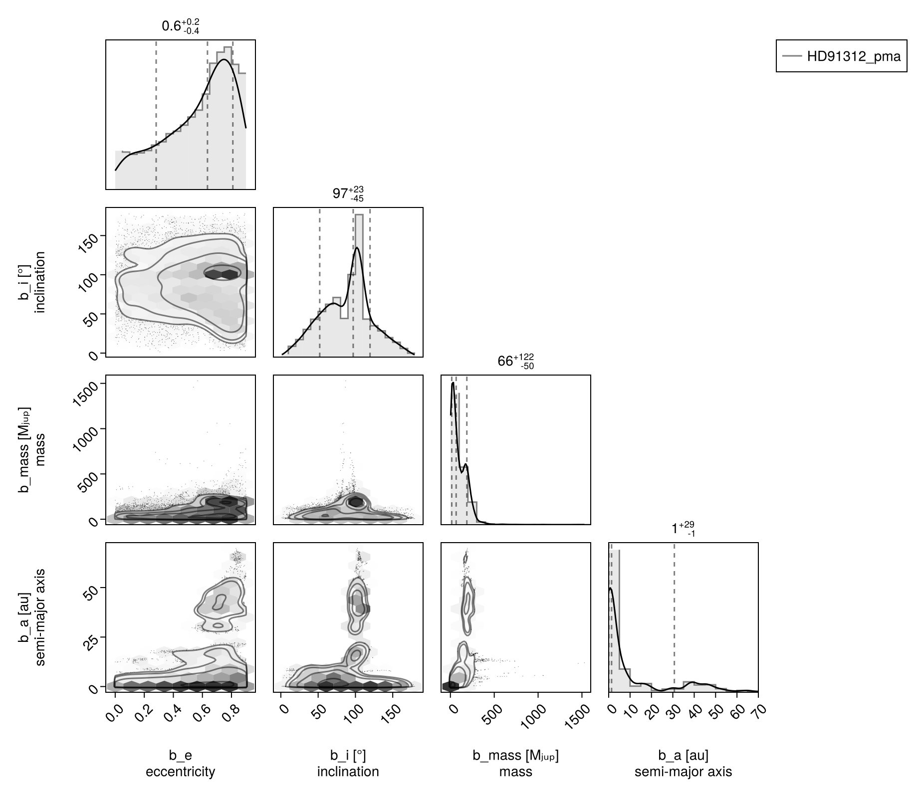
Notice how there are completely separated peaks? The default Octofitter sample (Hamiltonian Monte Carlo) is capabale of jumping 2-3σ gaps between modes, but such widely separated peaks can cause issues (hence why we used Pigeons in this example).
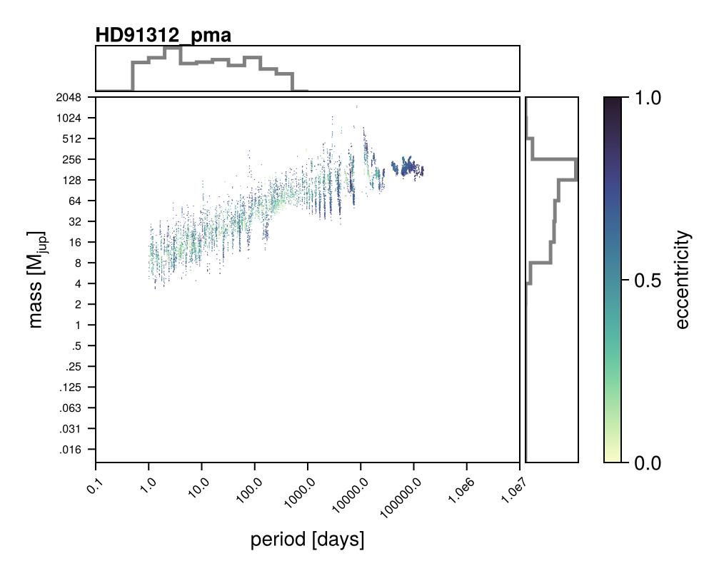
Posterior Mass vs. Semi-Major Axis
Given that this posterior is quite unconstrained, it is useful to make a simplified plot marginalizing over all orbital parameters besides separation. We can do this using dotplot:
using CairoMakie
Octofitter.dotplot(model_pma, chain_pma, mode=:period)