Basic RV Fit
You can use Octofitter to fit radial velocity data, either alone or in combination with other kinds of data. Multiple instruments (any number) are supported, as are arbitrary trends, and gaussian processes to model stellar activity.
Radial velocity modelling is supported in Octofitter via the extension package OctofitterRadialVelocity. To install it, run pkg> add OctofitterRadialVelocity
For this example, we will fit the orbit of the planet K2-131, and reproduce this RadVel tutorial.
We will use the following packages:
using Octofitter
using OctofitterRadialVelocity
using PlanetOrbits
using CairoMakie
using PairPlots
using CSV
using DataFrames
using Distributions
We will start by downloading and preparing a table of radial velocity measurements, and create a StarAbsoluteRVObs object to hold them.
The following functions allow you to directly load data from various public RV databases:
HARPS_DR1_rvs("star-name")HARPS_RVBank_observations("star-name")Lick_rvs("star-name")HIRES_rvs("star-name")
Make sure to credit the sources using the citation printed when you first access the catalog. Calling those functions with the name of a star will return a StarAbsoluteRVObs table.
If you would like to manually specify RV data, use the following format:
rv_data = Table(
     # epoch is in units of MJD. `jd2mjd` is a helper function to convert.
    # you can also put `years2mjd(2016.1231)`.
    # rv and σ_rv are in units of meters/second
    epoch=jd2mjd.([2455110.97985, 2455171.90825]),
    rv=[-6.54, -3.33],
    σ_rv=[1.30, 1.09]
)

rv_obs = StarAbsoluteRVObs(rv_data,
    name="insert name here",
    variables=@variables begin
        offset ~ Uniform(-1000, 1000) # m/s
        jitter ~ LogUniform(0.01, 10) # m/s
    end
)
Basic Fit
For this example, to replicate the results of RadVel, we will download their example data for K2-131 and format it for Octofitter:
rv_file = download("https://raw.githubusercontent.com/California-Planet-Search/radvel/master/example_data/k2-131.txt")
rv_dat_raw = CSV.read(rv_file, DataFrame, delim=' ')
rv_dat = DataFrame();
rv_dat.epoch = jd2mjd.(rv_dat_raw.time)
rv_dat.rv = rv_dat_raw.mnvel
rv_dat.σ_rv = rv_dat_raw.errvel
tels = sort(unique(rv_dat_raw.tel))

# This table includes data from two insturments. We create a separate
# likelihood object for each:
rvlike_harps = StarAbsoluteRVObs(
    rv_dat[rv_dat_raw.tel .== "harps-n",:],
    name="harps-n",
    variables=@variables begin
        offset ~ Normal(-6693,100) # m/s
        jitter ~ LogUniform(0.1,100) # m/s
    end
)
rvlike_pfs = StarAbsoluteRVObs(
    rv_dat[rv_dat_raw.tel .== "pfs",:],
    name="pfs",
    variables=@variables begin
        offset ~ Normal(0,100) # m/s
        jitter ~ LogUniform(0.1,100) # m/s
    end
)
StarAbsoluteRVObs Table with 3 columns and 31 rows:
epoch rv σ_rv
┌──────────────────────
1 │ 57828.4 -45.17 3.88
2 │ 57828.4 -36.47 4.03
3 │ 57829.2 -20.52 3.55
4 │ 57829.2 -4.58 6.07
5 │ 57830.1 17.71 3.56
6 │ 57830.1 23.34 3.48
7 │ 57830.2 21.34 3.51
8 │ 57830.2 19.92 3.26
9 │ 57830.2 -0.74 3.44
10 │ 57830.3 16.9 3.5
11 │ 57830.3 8.25 4.64
12 │ 57830.4 -4.06 4.91
13 │ 57832.1 -29.51 4.96
14 │ 57832.1 -21.56 4.11
15 │ 57832.2 -25.76 5.59
16 │ 57833.1 2.1 3.91
17 │ 57833.1 4.38 3.73
⋮ │ ⋮ ⋮ ⋮Now, create a planet. We can use the RadialVelocityOrbit type from PlanetOrbits.jl that requires fewer parameters (eg no inclination or longitude of ascending node). We could instead use a Visual{KepOrbit} or similar if we wanted to include these parameters and visualize the orbit in the plane of the sky.
planet_1 = Planet(
    name="b",
    basis=RadialVelocityOrbit,
    observations=[],
    variables=@variables begin
        e = 0
        ω = 0.0
        # To match RadVel, we set a prior on Period and calculate semi-major axis from it
        P ~ truncated(
            Normal(0.3693038/365.256360417, 0.0000091/365.256360417),
            lower=0.0001
        )
        M = system.M
        a = cbrt(M * P^2) # note the equals sign.
        τ ~ UniformCircular(1.0)
        tp = τ*P*365.256360417 + 57782 # reference epoch for τ. Choose an MJD date near your data.
        # minimum planet mass [jupiter masses]. really m*sin(i)
        mass ~ LogUniform(0.001, 10)
    end
)

sys = System(
    name = "k2_132",
    companions=[planet_1],
    observations=[rvlike_harps, rvlike_pfs],
    variables=@variables begin
        M ~ truncated(Normal(0.82, 0.02),lower=0.1) # (Baines & Armstrong 2011).
    end
)
System model k2_132
Derived:
Priors:
M ~ Truncated(Distributions.Normal{Float64}(μ=0.82, σ=0.02); lower=0.1)
Planet b
Derived:
τ = (atan(τy, τx) / (2π)) * 1.0
e = 0
ω = 0.0
M = system.M
a = cbrt(M * P ^ 2)
tp = τ * P * 365.256360417 + 57782
Priors:
P ~ Truncated(Distributions.Normal{Float64}(μ=0.001011081092683449, σ=2.4914008313533153e-8); lower=0.0001)
τx ~ Distributions.Normal{Float64}(μ=0.0, σ=1.0)
τy ~ Distributions.Normal{Float64}(μ=0.0, σ=1.0)
mass ~ Distributions.LogUniform{Float64}(a=0.001, b=10.0)
Octofitter.UnitLengthPrior{:τx, :τy}: √(τx^2+τy^2) ~ LogNormal(log(1), 0.02)
StarAbsoluteRVObs Table with 3 columns and 39 rows:
epoch rv σ_rv
┌─────────────────────────
1 │ 57782.2 -6682.78 3.71
2 │ 57783.1 -6710.55 5.95
3 │ 57783.2 -6698.96 8.76
4 │ 57812.1 -6672.32 4.0
5 │ 57812.2 -6672.0 4.22
6 │ 57812.2 -6690.31 4.63
7 │ 57813.0 -6701.27 4.12
8 │ 57813.1 -6700.71 5.34
9 │ 57813.1 -6695.97 3.67
10 │ 57813.1 -6705.87 4.23
11 │ 57813.1 -6694.27 5.12
12 │ 57813.2 -6699.99 5.0
13 │ 57813.2 -6696.17 10.43
14 │ 57836.0 -6675.4 7.03
15 │ 57836.0 -6665.92 7.48
16 │ 57836.0 -6661.9 6.03
17 │ 57836.1 -6657.92 5.08
⋮ │ ⋮ ⋮ ⋮StarAbsoluteRVObs Table with 3 columns and 31 rows:
epoch rv σ_rv
┌──────────────────────
1 │ 57828.4 -45.17 3.88
2 │ 57828.4 -36.47 4.03
3 │ 57829.2 -20.52 3.55
4 │ 57829.2 -4.58 6.07
5 │ 57830.1 17.71 3.56
6 │ 57830.1 23.34 3.48
7 │ 57830.2 21.34 3.51
8 │ 57830.2 19.92 3.26
9 │ 57830.2 -0.74 3.44
10 │ 57830.3 16.9 3.5
11 │ 57830.3 8.25 4.64
12 │ 57830.4 -4.06 4.91
13 │ 57832.1 -29.51 4.96
14 │ 57832.1 -21.56 4.11
15 │ 57832.2 -25.76 5.59
16 │ 57833.1 2.1 3.91
17 │ 57833.1 4.38 3.73
⋮ │ ⋮ ⋮ ⋮
Note how the rvlike object was attached to the k2_132 system instead of the planet. This is because the observed radial velocity is of the star, and is caused by any/all orbiting planets.
The rv0 and jitter parameters specify priors for the instrument-specific offset and white noise jitter standard deviation. The _i index matches the inst_idx used to create the observation table.
Note also here that the mass variable is really msini, or the minimum mass of the planet.
We can now prepare our model for sampling.
model = Octofitter.LogDensityModel(sys)LogDensityModel for System k2_132 of dimension 9 and 71 epochs with fields .ℓπcallback and .∇ℓπcallback
Initialize the starting points, and confirm the data are entered correcly:
init_chain = initialize!(model)

using CairoMakie
fig = Octofitter.rvpostplot(model, init_chain)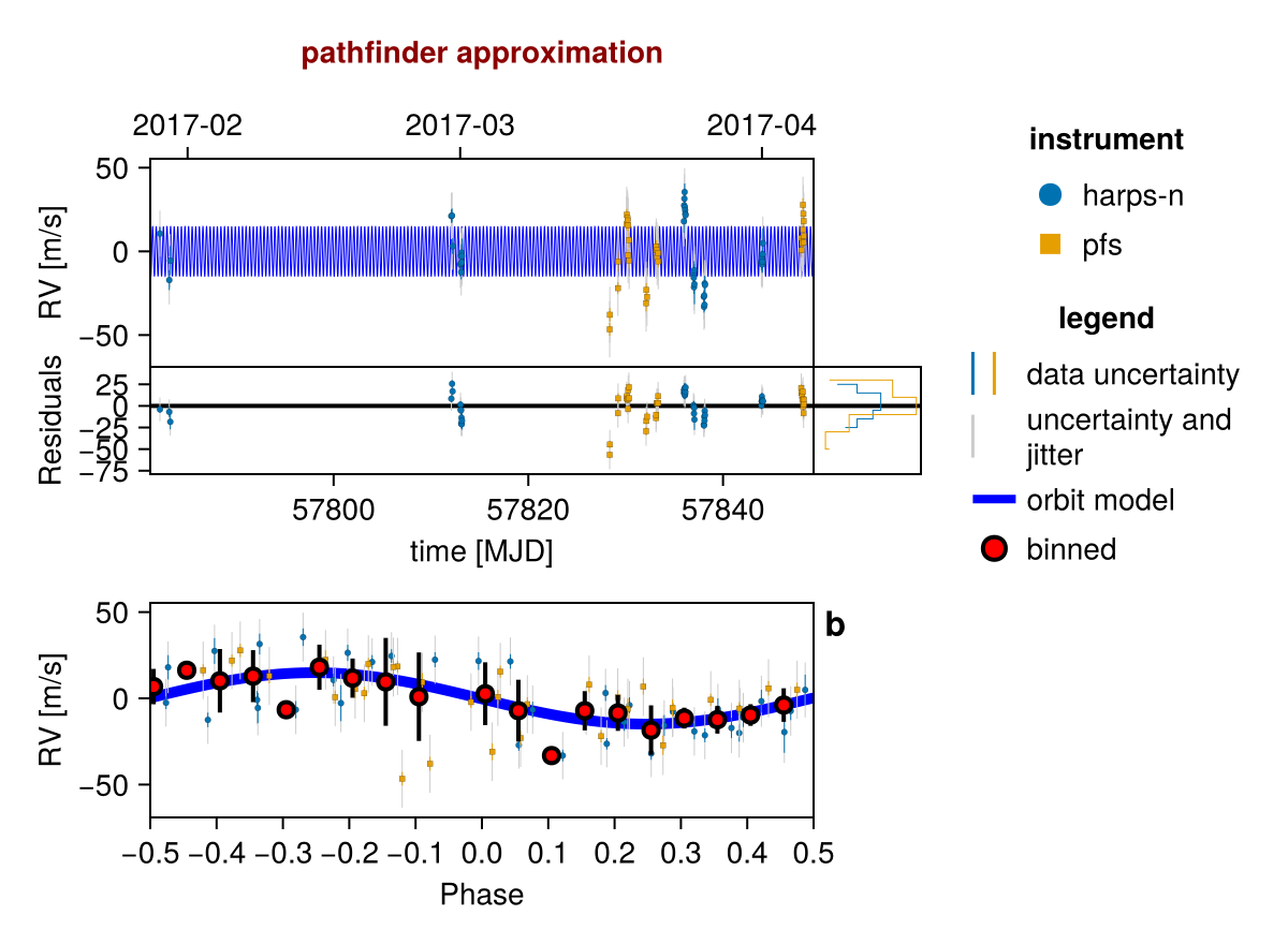
Sample:
using Random
rng = Random.Xoshiro(0)

chain = octofit(rng, model)
Chains MCMC chain (1000×28×1 Array{Float64, 3}):
Iterations = 1:1:1000
Number of chains = 1
Samples per chain = 1000
Wall duration = 21.06 seconds
Compute duration = 21.06 seconds
parameters = M, harps_n_offset, harps_n_jitter, pfs_offset, pfs_jitter, b_P, b_τx, b_τy, b_mass, b_τ, b_e, b_ω, b_M, b_a, b_tp
internals = n_steps, is_accept, acceptance_rate, hamiltonian_energy, hamiltonian_energy_error, max_hamiltonian_energy_error, tree_depth, numerical_error, step_size, nom_step_size, is_adapt, loglike, logpost, tree_depth, numerical_error
Use `describe(chains)` for summary statistics and quantiles.
Excellent! Let's plot an orbit sampled from the posterior:
using CairoMakie
fig = Octofitter.rvpostplot(model, chain) # saved to "k2_132-rvpostplot.png"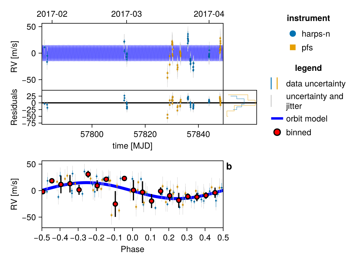
We can also plot a sample of draws from the posterior:
using CairoMakie: Makie
octoplot(model, chain)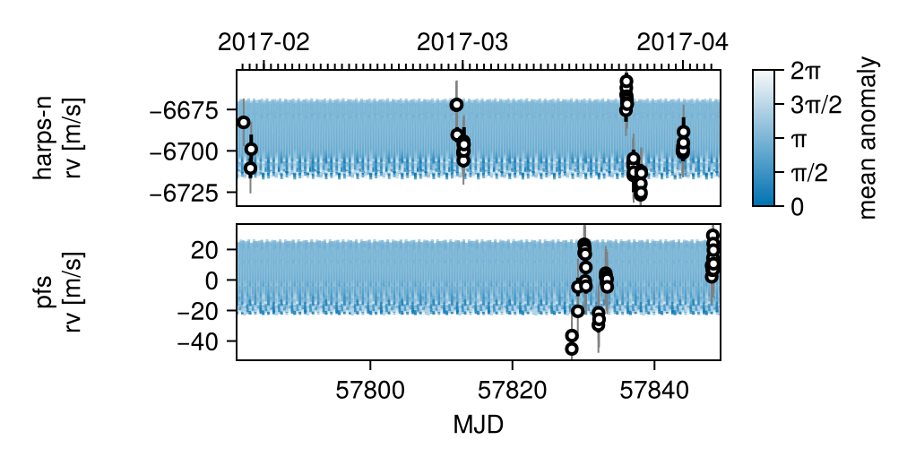
And create a corner plot:
using PairPlots, CairoMakie
octocorner(model, chain)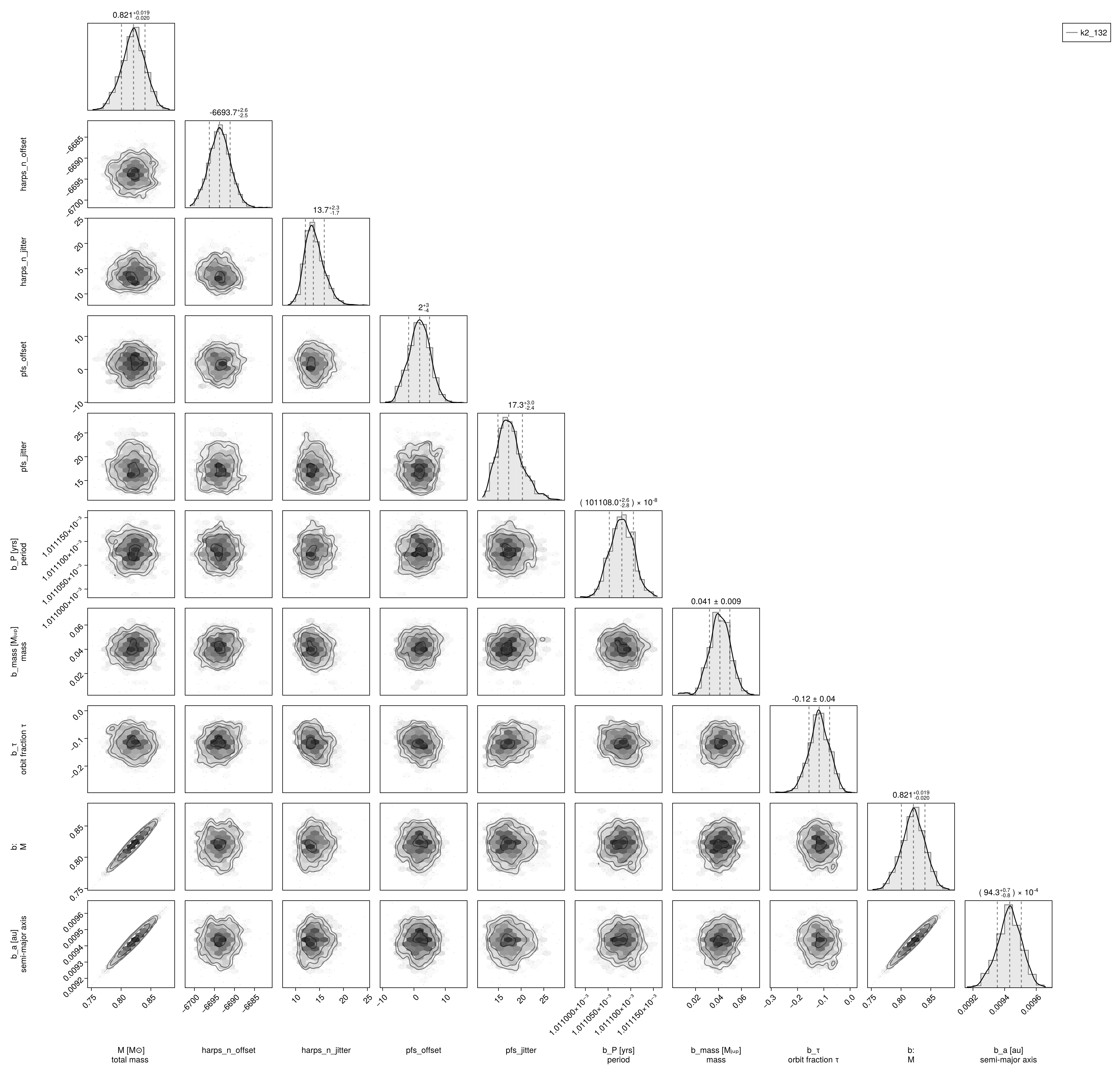
This example continues in Fit Gaussian Process.
Simulating RV Data
To generate synthetic radial velocity data for testing, the recommended approach is to use Octofitter's built-in simulation capabilities. See the Generating and Fitting Simulated Data tutorial for a complete guide on simulating data from models.
Alternatively, you can generate RV data directly using the radvel function from PlanetOrbits.jl:
using PlanetOrbits

# Create an orbit
orb = orbit(a=1.0, e=0.1, ω=0.5, M=1.0, tp=58000.0)

# Calculate radial velocity at a given epoch
# Units: epoch in MJD, mass in solar masses (not Jupiter masses!)
epoch = 58100.0
companion_mass_msol = 0.001  # ~1 Jupiter mass in solar masses
rv = radvel(orb, epoch, companion_mass_msol)  # returns m/s