Fitting Images

One of the key features of Octofitter.jl is the ability to search for planets directly from images of the system. Sampling from images is much more computationally demanding than sampling from astrometry, but it allows for a few very powerful results:

1. You can search for a planet that is not well detected in a single image. By this, we mean you can feed in images of a system with no clear detections, and see if a planet is hiding in the noise based off of its Kepelerian motion.

2. Not detecting a planet in a given image can be almost as useful as a detection for constraining its orbit. If you have a clear detection in one epoch, but no detection in another, Octofitter can use the image from the second epoch to rule out large swathes of possible orbits.

Sampling from images can be freely combined with any known astrometry points, as well as astrometric acceleration. See advanced models for more details.

Preparing images

The first step will be to load your images. For this, we will use our AstroImages.jl package.

Start by loading your images:

using Octofitter
using OctofitterImages
using Distributions
using AstroImages
using CairoMakie
using Pigeons

# Load individual iamges
# image1 = load("image1.fits")
# image2 = load("image2.fits")

# Or slices from a cube:
# cube = load("cube1.fits")
# image1 = cube[:,:,1]

# Download sample images from GitHub
download(
    "https://github.com/sefffal/Octofitter.jl/raw/main/docs/image-examples-1.fits",
    "image-examples-1.fits"
)

# Or multi-extension FITS (this example)
images = AstroImages.load("image-examples-1.fits",:)

5-element Vector{AstroImages.AstroImageMat{Float64, Tuple{DimensionalData.Dimensions.X{DimensionalData.Dimensions.Lookups.Sampled{Int64, Base.OneTo{Int64}, DimensionalData.Dimensions.Lookups.ForwardOrdered, DimensionalData.Dimensions.Lookups.Regular{Int64}, DimensionalData.Dimensions.Lookups.Points, DimensionalData.Dimensions.Lookups.NoMetadata}}, DimensionalData.Dimensions.Y{DimensionalData.Dimensions.Lookups.Sampled{Int64, Base.OneTo{Int64}, DimensionalData.Dimensions.Lookups.ForwardOrdered, DimensionalData.Dimensions.Lookups.Regular{Int64}, DimensionalData.Dimensions.Lookups.Points, DimensionalData.Dimensions.Lookups.NoMetadata}}}, Tuple{}, Matrix{Float64}, Tuple{DimensionalData.Dimensions.X{DimensionalData.Dimensions.Lookups.Sampled{Int64, Base.OneTo{Int64}, DimensionalData.Dimensions.Lookups.ForwardOrdered, DimensionalData.Dimensions.Lookups.Regular{Int64}, DimensionalData.Dimensions.Lookups.Points, DimensionalData.Dimensions.Lookups.NoMetadata}}, DimensionalData.Dimensions.Y{DimensionalData.Dimensions.Lookups.Sampled{Int64, Base.OneTo{Int64}, DimensionalData.Dimensions.Lookups.ForwardOrdered, DimensionalData.Dimensions.Lookups.Regular{Int64}, DimensionalData.Dimensions.Lookups.Points, DimensionalData.Dimensions.Lookups.NoMetadata}}}}}:
 [-0.340230578841865 -0.31239887526186355 … -0.2903753168231458 -0.34686827004814064; -0.29826568928566355 -0.27872689920999305 … -0.246452640103626 -0.2873140658333837; … ; 0.2673577868138141 0.2674003307584391 … -0.35696041486602914 -0.4320582965232348; 0.34147717271077094 0.3420908537177248 … -0.3358061981896538 -0.4139117427343716]
 [-1.0477769487233675 -0.903332487139985 … 1.4299602191511185 1.5070937596027922; -0.9888724404777535 -0.8589483767137767 … 1.1201264194935676 1.1803510698319304; … ; -0.43042419506343155 -0.46545013356425746 … -0.7066171674807686 -0.8619933383603304; -0.5837006039738425 -0.6021768042432977 … -0.8745923304009366 -1.0622653729194567]
 [-1.3673176596472436 -1.1985348376204175 … 1.1486692344915643 1.2929199629807906; -1.1143572848991925 -0.9810874969329584 … 0.9739105840286464 1.079311141942771; … ; 1.0292715351056276 0.8022139684685823 … 0.674123592556085 0.8519386886571362; 1.2170463982677187 0.9582307659215409 … 0.7602550494569255 0.959778160219427]
 [-0.16664741987337547 -0.13437529569419648 … -1.2963013699793633 -1.413565369547865; -0.2149990713151032 -0.1847368741065949 … -1.0549153738841368 -1.1490484959706464; … ; -0.5872462145987273 -0.5703179209210852 … 0.19469039731388912 0.31932314143450863; -0.7173113967617594 -0.6848676990867931 … 0.19122281859925802 0.3434506497145075]
 [0.47470453920043826 0.4747486393369815 … -0.16662161045865695 -0.16297895606178783; 0.4078627130832368 0.4041383409077344 … -0.18122203442704718 -0.17883512905931084; … ; 0.07003384675445126 0.19916060264117244 … -0.44137489323835993 -0.5253547777211444; 0.023766763613137065 0.1809119688664255 … -0.5699244785815155 -0.6776496918698217]

You can preview the image using imview from AstroImages:

# imshow2(image1, cmap=:magma) # for a single image
hcat(imview.(images, clims=(-1.0, 4.0))...)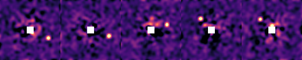

Your images should either be convolved with a gaussian of diameter one λ/D, or be matched filtered. This is so that the values of the pixels in the image represent the photometry at that location.

If you want to perform the convolution in Julia, see ImageFiltering.jl.

Build the model

First, we create a table of our image observations:

image_dat = Table(;
    epoch = 56000 .+ [1238.6, 1584.7, 3220.0, 7495.9, 7610.4],
    image = [
        AstroImages.recenter(images[1]),
        AstroImages.recenter(images[2]),
        AstroImages.recenter(images[3]),
        AstroImages.recenter(images[4]),
        AstroImages.recenter(images[5])
    ],
    platescale = [10.0, 10.0, 10.0, 10.0, 10.0]
)

Provide one entry for each image you want to sample from. platescale should be the pixel scale of your images, in milliarseconds / pixel. epoch should be the Modified Julian Day (MJD) that your image was taken; you can use the mjd("2021-09-09") function to calculate this for you. (The sample images above ship with arbitrary epoch labels spanning about 17 years, so we offset them onto plausible MJDs. Only the spacing of the epochs affects the fit.)

Areas of the image where there is no data should be filled with NaN and will not contribute to the likelihood of your model.

Each image must be re-centered so that index [0,0] falls on the position of ref — the body the images are measured against, usually the host star. That is what AstroImages.recenter is doing above.

Now the bodies. The host star A is a body like any other, and the planet b orbits it (about=A):

A = Body(
    name="A",
    variables=@variables begin
        mass ~ truncated(Normal(2.0, 0.1), lower=0.1) # M⊙
    end
)

b = Body(
    name="b",
    about=A,
    variables=@variables begin
        # Brightness of this planet in the H band, in image units.
        flux_H ~ Normal(3.8, 0.5)

        a ~ truncated(Normal(13, 4), lower=0.1, upper=100)
        e ~ Uniform(0.0, 0.5)
        i ~ Sine()
        ω ~ UniformCircular()
        Ω ~ UniformCircular()
        θ ~ UniformCircular()       # position angle at `epoch`
        epoch = 57238.6             # reference epoch for θ; near the first image
    end
)

See Fit Relative Astrometry for a description of the different orbital parameters, and conventions used.

Finally the observation itself, and the system:

image_obs = ImageObs(
    image_dat,
    targets = (b,),        # every source these images are modelled to contain
    ref     = A,           # the point index [0,0] of each image sits on
    band    = :H,          # read each target's `flux_H` variable
    name    = "SPHERE",
    variables=@variables begin
        # The following are optional parameters for marginalizing over instrument systematics:
        # Platescale uncertainty multiplier [could use: platescale ~ truncated(Normal(1, 0.01), lower=0)]
        platescale = 1.0
        # North angle offset in radians [could use: northangle ~ Normal(0, deg2rad(1))]
        northangle = 0.0
    end
)

sys = System(
    name="HD82134",
    bodies=[A, b],
    observations=[image_obs],
    variables=@variables begin
        plx ~ truncated(Normal(45., 0.02), lower=0.1)
    end
)

[ Info: Measuring contrast from image
[ Info: [HD82134] observing_geometry = true (auto): no observation can report comparable predictions (ImageObs); nothing to measure, so keeping the correction on — no draws needed (seed 0xc70f177e5000001)
[ Info: [HD82134] barycentric_lighttime = true (auto): no observation can report comparable predictions (ImageObs); nothing to measure, so keeping the correction on — no draws needed (seed 0xc70f177e5000001)

Planet Flux Variables

Each body you want to model should have a flux_<band> variable, e.g. flux_H.

c = Body(name="c", about=A, variables=@variables begin
    flux_H ~ Normal(1.2, 0.5)
    a ~ truncated(Normal(30, 8), lower=0.1, upper=100)
    # ... the rest of c's orbit ...
end)

image_obs = ImageObs(image_dat; targets=(b, c), ref=A, band=:H, name="SPHERE")

A few consequences worth knowing:

• band=:H selects which flux_<band> variable each target is read from. You may omit band= only when the bodies declare exactly one band (a bare flux = ...); with several bands defined and no band=, you get an error listing them.
• The units of flux_H are the units of your image pixels — contrast, magnitudes, Jy, or arbitrary, as long as they are consistent. Setting the host's flux_H = 1.0 makes every other body's flux a contrast ratio, but for images the host is usually not in targets at all (it is behind the coronagraph), so it needs no flux variable.
• targets is a structural statement about which sources the forward model contains. It is deliberately not inferred from "every body with a flux in this band": leaving c out is a different model from including c with a flux prior pushed near zero.
• ref is what the image is centred against. ref=Barycentre and ref=b (one companion measured against another) are both legal, and useful for hierarchical stellar systems.

By default, the contrast of the images is calculated automatically, but you can supply your own contrast curve as well by also passing a contrast column: contrast=OctofitterImages.contrast_interp(AstroImages.recenter(my_image)). That callable maps separation in pixels to the 1σ flux uncertainty there. A 2-D contrastmap column is honoured too.

You can freely mix and match images from different instruments as long as you specify the correct platescale — one ImageObs per instrument. You can also provide images from multiple bands and they will be sampled independently. If you wish to tie them together, see Connecting Mass with Photometry.

You can also do some very clever things like searching for planets that are co-planar and/or have a specific resonance between their periods. To do this, put the period of the system or base period in the system variables and derive the body variables from those values of the system.

Sampling

Sampling from images is much more challenging than relative astrometry or proper motion anomaly, so the fitting process tends to take longer.

This is because the posterior is much "bumpier" with images. One way this manifests is very high tree depths. You might see a sampling report that says max_tree_depth_frac = 0.9 or even 1.0. To encourage the sampler to take larger steps and explore the images, it's recommended to lower the target acceptance ratio to around 0.5±0.2 and also increase the number of adapataion steps.

model = Octofitter.LogDensityModel(sys)

chain, pt = octofit_pigeons(model, n_rounds=10)
display(chain)

[ Info: Preparing model
┌ Info: Determined number of free variables
└   D = 12
┌ Info: Determined number type
└   T = Float64
ℓπcallback(θ): 0.000014 seconds
∇ℓπcallback(θ): 0.000028 seconds (1 allocation: 32 bytes)
┌ Warning: This model has priors that cannot be sampled IID.
└ @ OctofitterPigeonsExt ~/octo-maintenance/runner/actions-runner/_work/Octofitter.jl/Octofitter.jl/ext/OctofitterPigeonsExt.jl:192
[ Info: Sampler running with multiple threads     : true
[ Info: Likelihood evaluated with multiple threads: false
[ Info: [HD82134] observing_geometry = true (user)
[ Info: [HD82134] barycentric_lighttime = true (user)
[ Info: [HD82134] observing_geometry = true (user)
[ Info: [HD82134] barycentric_lighttime = true (user)
┌ Info: Starting values not provided for all parameters! Guessing starting point using global optimization:
│   num_params = 12
└   num_fixed = 0
┌ Warning: Verbosity toggle: unrecognized_stop_reason
│  Unrecognized stop reason: Too many steps (101) without any function evaluations (probably search has converged). Defaulting to ReturnCode.Default.
└ @ OptimizationBase ~/.julia/packages/OptimizationBase/Jfw5O/src/utils.jl:170
┌ Warning: Pathfinder error: MethodError(copy, (SplittableRandoms.SplittableRandom(0x2636cfbad22366f5, 0xaabf13ae126f9159),), 0x000000000000ab8d)
└ @ Octofitter ~/octo-maintenance/runner/actions-runner/_work/Octofitter.jl/Octofitter.jl/src/initialization.jl:944
┌ Warning: Using BBO result as fallback
└ @ Octofitter ~/octo-maintenance/runner/actions-runner/_work/Octofitter.jl/Octofitter.jl/src/initialization.jl:945
┌ Info: Found sample of initial positions
│   logpost_range = (93.2574024996936, 93.2574024996936)
└   mean_logpost = 93.25740249969357
────────────────────────────────────────────────────────────────────────────────────────────────────────────────────────
  scans     restarts      Λ        Λ_var      time(s)    allc(B)  log(Z₁/Z₀)   min(α)     mean(α)    min(αₑ)   mean(αₑ)
────────── ────────── ────────── ────────── ────────── ────────── ────────── ────────── ────────── ────────── ──────────
        2          0        3.1       2.95       1.13   5.43e+06       78.4   4.63e-07      0.805          1          1
        4          0       3.23       6.07     0.0852   1.99e+05       74.2     0.0104        0.7          1          1
        8          0       4.17       4.15      0.177    3.8e+05         70     0.0476      0.732          1          1
       16          0       4.07       4.73      0.346   6.86e+05       68.8      0.196      0.716          1          1
       32          0       4.41       4.61      0.674    1.1e+06       66.9      0.326      0.709          1          1
       64          2       4.38       3.53       2.05   6.08e+07       64.2      0.165      0.745          1          1
      128          5       4.62       3.55       2.78   1.02e+08       64.7      0.382      0.737          1          1
      256         19       4.51       3.63       5.53   2.01e+08       64.7      0.502      0.738          1          1
      512         34       4.64       4.47         11   3.98e+08       64.3      0.577      0.706          1          1
 1.02e+03         70       4.57       4.02         22    7.9e+08       64.8      0.553      0.723          1          1
────────────────────────────────────────────────────────────────────────────────────────────────────────────────────────

Diagnostics

The first thing you should do with your results is check a few diagnostics to make sure the sampler converged as intended.

The acceptance rate should be somewhat lower than when fitting just astrometry, e.g. around the 0.6 target.

You can make a trace plot:

lines(
    chain["b_a"][:],
    axis=(;
        xlabel="iteration",
        ylabel="semi-major axis (aU)"
    )
)

And an auto-correlation plot:

using StatsBase
lines(
    autocor(chain["b_e"][:], 1:500),
    axis=(;
        xlabel="lag",
        ylabel="autocorrelation",
    )
)

For this model, there is somewhat higher correlation between samples. Some thinning to remove this correlation is recommended.

Analysis

We can now view the orbit fit:

octoplot(model, chain)

octoplot returns an OctoPlotResult, which carries the figure itself plus a named tuple of the axes it built. That is what lets us reach into the sky panel and draw underneath the orbits:

res = octoplot(model, chain)
fig = res.figure
ax = res.axes.sky.sky   # the sky-plane axis

# We have to do some annoying work to get the image orientated correctly,
# since we want the RA axis increasing to the left.
image_idx = 2
platescale = image_dat.platescale[image_idx]
img = AstroImages.recenter(AstroImage(collect(image_dat.image[image_idx])[end:-1:begin,:]))
imgax1 = dims(img,1) .* platescale
imgax2 = dims(img,2) .* platescale
h = heatmap!(ax, imgax1, imgax2, collect(img), colormap=:greys)
Makie.translate!(h, 0,0,-1) # Send heatmap to back of the plot

# Add colorbar for image
Colorbar(fig[1,2], h, label="image flux")

Makie.resize_to_layout!(fig)
fig

Another useful view would be the orbits over a stack of the maximum pixel values of all images.

res = octoplot(model, chain)
fig = res.figure
ax = res.axes.sky.sky

# We have to do some annoying work to get the image orientated correctly
# since we want the RA axis increasing to the left.
platescale = image_dat.platescale[image_idx]
imgs = maximum(stack(image_dat.image),dims=3)[:,:]
img = AstroImages.recenter(AstroImage(imgs[end:-1:begin,:]))
imgax1 = dims(img,1) .* platescale
imgax2 = dims(img,2) .* platescale
h = heatmap!(ax, imgax1, imgax2, collect(img), colormap=:greys)
Makie.translate!(h, 0,0,-1) # Send heatmap to back of the plot
Makie.resize_to_layout!(fig)
fig

Pair Plot

We can show the relationships between variables on a pair plot (aka corner plot):

using CairoMakie, PairPlots
octocorner(model, chain, small=true)

Note that this time, we also show the recovered photometry in the corner plot.

Assessing Detections

To assess a detection, we can treat all the orbital variables as nuisance parameters. We start by plotting the marginal distribution of the flux parameter, flux_H:

Body variables are named <body>_<variable> in the chain, so the planet's H-band flux is b_flux_H.

hist(chain["b_flux_H"][:], axis=(xlabel="flux", ylabel="counts"))

We can calculate an analog of the traditional signal to noise ratio (SNR) using that same histogram:

flux = chain["b_flux_H"]
snr = mean(flux)/std(flux)

14.24843262204144

It might be better to consider a related measure, like the median flux over the interquartile distance. This will depend on your application.