Hierarchical Co-Planar, Near-Resonant Model
This example shows how you can fit a two planet model to relative astrometry data. This functionality would work equally well with RV, images, etc.
We will demonstrate two models: the first, where the planets are exactly co-planar (using a single set of variables for the inlination and position angle of ascending node for both planets), and a second, where the planets are approximately co-planar according to a custom prior.
using Octofitter
using CairoMakie
using PairPlots
using Distributions
using PlanetOrbits
using Pigeons
Data
For this example, we will use astrometry from the HR8799 system collated by Jason Wang and retrieved from the website Whereistheplanet.com.
Specify the data here. We'll wrap it in observation objects below.
astrom_dat_b = Table(;
    epoch = [53200.0, 54314.0, 54398.0, 54727.0, 55042.0, 55044.0, 55136.0, 55390.0, 55499.0, 55763.0, 56130.0, 56226.0, 56581.0, 56855.0, 58798.03906, 59453.245, 59454.231],
    ra    = [1471.0, 1504.0, 1500.0, 1516.0, 1526.0, 1531.0, 1524.0, 1532.0, 1535.0, 1541.0, 1545.0, 1549.0, 1545.0, 1560.0, 1611.002, 1622.924, 1622.872],
    dec   = [887.0, 837.0, 836.0, 818.0, 797.0, 794.0, 795.0, 783.0, 766.0, 762.0, 747.0, 743.0, 724.0, 725.0, 604.893, 570.534, 571.296],
    σ_ra  = [6.0, 3.0, 7.0, 4.0, 4.0, 7.0, 10.0, 5.0, 15.0, 5.0, 5.0, 4.0, 22.0, 13.0, 0.133, 0.32, 0.204],
    σ_dec = [6.0, 3.0, 7.0, 4.0, 4.0, 7.0, 10.0, 5.0, 15.0, 5.0, 5.0, 4.0, 22.0, 13.0, 0.199, 0.296, 0.446],
    cor   = [0.0, 0.0, 0.0, 0.0, 0.0, 0.0, 0.0, 0.0, 0.0, 0.0, 0.0, 0.0, 0.0, 0.0, -0.406, -0.905, -0.79]
)

astrom_dat_c = Table(;
    epoch = [53200.0, 54314.0, 54398.0, 54727.0, 55042.0, 55136.0, 55390.0, 55499.0, 55763.0, 56130.0, 56226.0, 56581.0, 56855.0],
    ra    = [-739.0, -683.0, -678.0, -663.0, -639.0, -636.0, -619.0, -607.0, -595.0, -578.0, -572.0, -542.0, -540.0],
    dec   = [612.0, 671.0, 678.0, 693.0, 712.0, 720.0, 728.0, 744.0, 747.0, 761.0, 768.0, 784.0, 799.0],
    σ_ra  = [6.0, 4.0, 7.0, 3.0, 4.0, 9.0, 4.0, 12.0, 4.0, 5.0, 3.0, 22.0, 12.0],
    σ_dec = [6.0, 4.0, 7.0, 3.0, 4.0, 9.0, 4.0, 12.0, 4.0, 5.0, 3.0, 22.0, 12.0],
    cor   = [0.0, 0.0, 0.0, 0.0, 0.0, 0.0, 0.0, 0.0, 0.0, 0.0, 0.0, 0.0, 0.0]
)
The bodies
HR 8799 b is the outer of the two planets and c the inner one, so we write the hierarchy as a Jacobi chain: c orbits the star, and b orbits the barycentre of the star and c (about=(A, c)).
A = Body(
    name="A",
    variables=@variables begin
        mass ~ truncated(Normal(1.5, 0.02), lower=0.1)   # [M⊙]
    end
)
Exact Co-Planar Model
This model will use a single pair of i and Ω variables for both planets to enforce exact co-planarity. Sharing a parameter between two bodies is done by hoisting it to the system block.
planet_c = Body(
    name="c",
    about=A,
    variables=@variables begin
        mass ~ Uniform(0, 12mjup)          # [M⊙]
        e = 0.0
        ω = 0.0

        # Use the system inclination and longitude of ascending node variables
        i = system.i
        Ω = system.Ω

        # Specify the period as ~ 10% around the P_nominal variable
        P_mul ~ truncated(Normal(1, 0.1), lower=0.1)
        P = system.P_nominal * P_mul * year2day_julian   # [days]

        θ ~ UniformCircular()
        epoch = 59454.231   # reference epoch for θ. Choose an MJD date near your data.
    end
)

planet_b = Body(
    name="b",
    about=(A, planet_c),                   # Jacobi: b orbits the A+c barycentre
    variables=@variables begin
        mass ~ Uniform(0, 12mjup)          # [M⊙]
        e = 0.0
        ω = 0.0

        i = system.i
        Ω = system.Ω

        # Specify the period as ~ 10% around 2X the P_nominal variable
        P_mul ~ Normal(1, 0.1)
        P = 2 * system.P_nominal * P_mul * year2day_julian   # [days]

        θ ~ UniformCircular()
        epoch = 59454.231
    end
)

# Show how the data connects with the model
astrom_b = RelAstromObs(
    astrom_dat_b;
    target = planet_b,
    ref = A,
    name = "GPI_b",
    variables = @variables begin
        # Fixed values for this example - could be free variables:
        jitter = 0        # mas [could use: jitter ~ Uniform(0, 10)]
        northangle = 0    # radians [could use: northangle ~ Normal(0, deg2rad(1))]
        platescale = 1    # relative [could use: platescale ~ truncated(Normal(1, 0.01), lower=0)]
    end
)

astrom_c = RelAstromObs(
    astrom_dat_c;
    target = planet_c,
    ref = A,
    name = "GPI_c",
    variables = @variables begin
        jitter = 0        # mas
        northangle = 0    # radians
        platescale = 1    # relative
    end
)

sys = System(
    name="HR8799_res_co",
    bodies=[A, planet_c, planet_b],
    observations=[astrom_b, astrom_c],
    variables=@variables begin
        plx ~ gaia_plx(;gaia_id=2832463659640297472)
        # We create inclination and longitude of ascending node variables at the
        # system level.
        i ~ Sine()
        Ω ~ UniformCircular()
        # We create a nominal period of planet c variable.
        P_nominal ~ Uniform(50, 300) # Julian years
    end
)

model = Octofitter.LogDensityModel(sys)
LogDensityModel for System HR8799_res_co of dimension 14 and 30 epochs with fields .ℓπcallback and .∇ℓπcallback
Let's plot our data before we start:
fig = scatter(astrom_dat_b.ra, astrom_dat_b.dec, axis=(;autolimitaspect=1))
scatter!(astrom_dat_c.ra, astrom_dat_c.dec)
scatter!([0], [0], marker='⋆', markersize=50, color=:black)
fig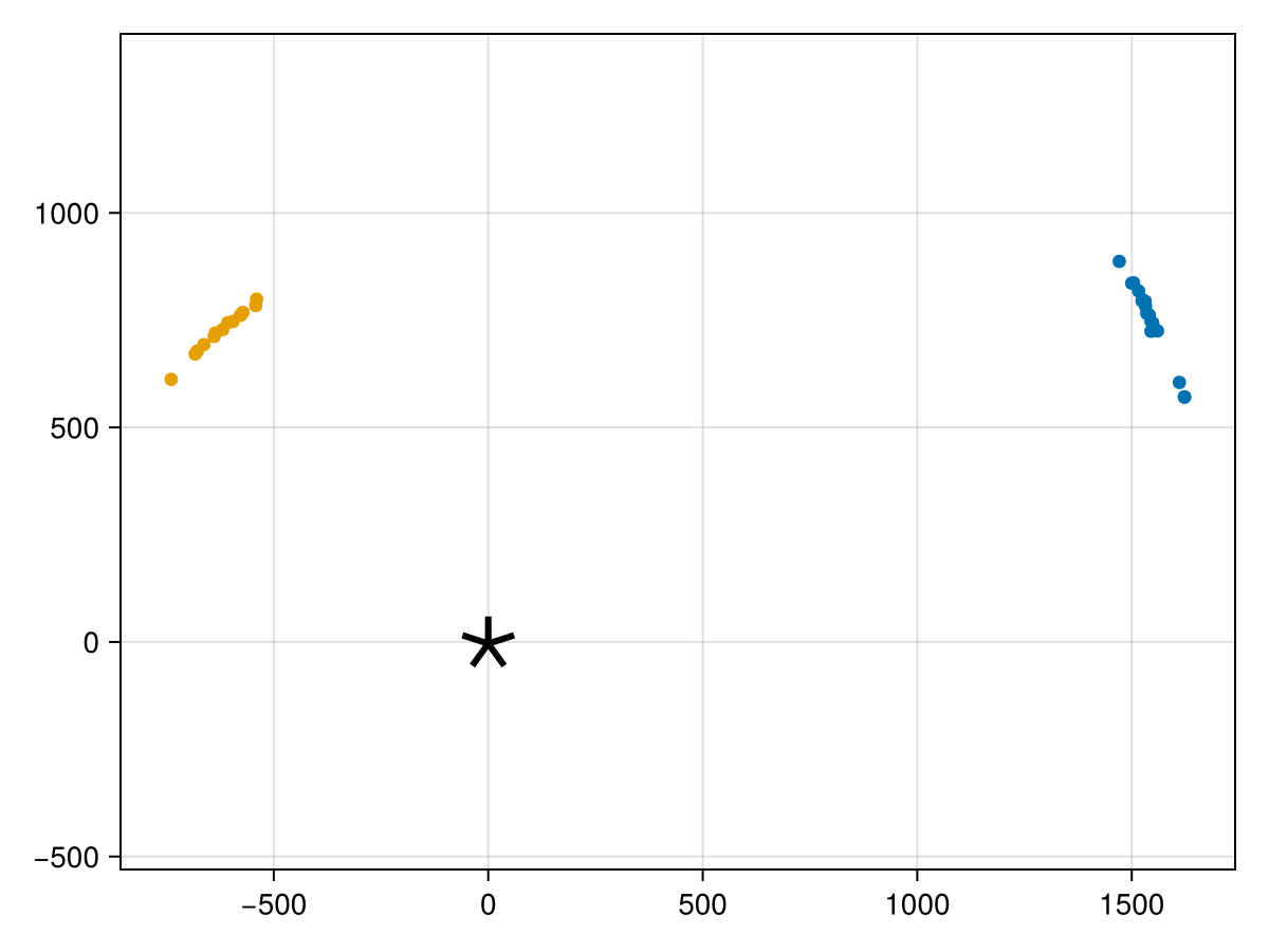
Initialize the starting points, and confirm the data are entered correcly:
init_chain = initialize!(model, (;
    plx = 24.4549,
    P_nominal = 230,
    bodies = (;
        A = (; mass = 1.48),
        b = (; mass = 5.73mjup),
        c = (; mass = 5.14mjup),
    )
))
octoplot(model, init_chain)
Now sample from the model using Pigeons parallel tempering:
results, pt = octofit_pigeons(model, n_rounds=10);┌ Warning: This model has priors that cannot be sampled IID.
└ @ OctofitterPigeonsExt ~/octo-maintenance/runner/actions-runner/_work/Octofitter.jl/Octofitter.jl/ext/OctofitterPigeonsExt.jl:192
[ Info: Sampler running with multiple threads : true
[ Info: Likelihood evaluated with multiple threads: false
[ Info: [HR8799_res_co] observing_geometry = true (user)
[ Info: [HR8799_res_co] barycentric_lighttime = false (user)
[ Info: [HR8799_res_co] observing_geometry = true (user)
[ Info: [HR8799_res_co] barycentric_lighttime = false (user)
────────────────────────────────────────────────────────────────────────────────────────────────────────────────────────
scans restarts Λ Λ_var time(s) allc(B) log(Z₁/Z₀) min(α) mean(α) min(αₑ) mean(αₑ)
────────── ────────── ────────── ────────── ────────── ────────── ────────── ────────── ────────── ────────── ──────────
2 0 3.18 1.87 1.75 1.06e+07 -1.03e+07 0 0.837 1 1
4 0 5.75 4.12 0.239 1.92e+06 -1.27e+06 0 0.681 1 1
8 0 5.41 5.71 0.47 3.92e+06 -4.19e+05 0 0.641 1 1
16 0 6.92 6.65 0.936 7.64e+06 -1.45e+05 0 0.562 1 1
32 0 6.61 7.68 1.88 1.52e+07 -2.05e+03 0 0.539 1 1
64 0 7.77 7.12 4.79 1.03e+08 -251 0 0.52 1 1
128 0 8.1 6.68 7.42 1.77e+08 -209 0 0.523 1 1
256 2 8.41 7.66 14.7 3.54e+08 -206 1.21e-57 0.482 1 1
512 5 9.14 8.25 29.3 6.98e+08 -205 3.08e-22 0.439 1 1
1.02e+03 16 9.58 8.69 58.6 1.37e+09 -205 6.2e-19 0.41 1 1
────────────────────────────────────────────────────────────────────────────────────────────────────────────────────────Plots the orbits:
octoplot(model, results)
Corner plot:
octocorner(model, results, small=true)
Now examine the period ratio:
hist(
    results[:b_P][:] ./ results[:c_P][:],
    axis=(;
        xlabel="period ratio",
        ylabel="counts",
    )
)
Approximately Co-Planar Model
We now set up two planets with their own separate i and Ω variables, calculate the mutual inclination, and add a prior that this mutual inclination is $0 \pm 10 \degree$. An oftern overlooked point is that that a half normal distribution on mutual inclination isn't going to actually peak at 0, more like $10 \degree$ because of how the priors on each planet's orbital plane interact.
Any expression ~ distribution line in a @variables block is a prior term, so the mutual-inclination constraint is written directly.
planet_c = Body(
    name="c",
    about=A,
    variables=@variables begin
        mass ~ Uniform(0, 12mjup)
        e = 0.0
        ω = 0.0

        i ~ Sine()
        Ω ~ UniformCircular()

        P_mul ~ truncated(Normal(1, 0.1), lower=0.1)
        P = system.P_nominal * P_mul * year2day_julian

        θ ~ UniformCircular()
        epoch = 59454.231
    end
)

planet_b = Body(
    name="b",
    about=(A, planet_c),
    variables=@variables begin
        mass ~ Uniform(0, 12mjup)
        e = 0.0
        ω = 0.0

        i~ Sine()
        Ω ~ UniformCircular()

        P_mul ~ Normal(1, 0.1)
        P = 2 * system.P_nominal * P_mul * year2day_julian

        θ ~ UniformCircular()
        epoch = 59454.231
    end
)

astrom_b = RelAstromObs(astrom_dat_b; target=planet_b, ref=A, name="GPI_b")
astrom_c = RelAstromObs(astrom_dat_c; target=planet_c, ref=A, name="GPI_c")

sys = System(
    name="HR8799_approx_res_co",
    bodies=[A, planet_c, planet_b],
    observations=[astrom_b, astrom_c],
    variables=@variables begin
        plx ~ gaia_plx(;gaia_id=2832463659640297472)

        # Calculate the mutual inclination
        mut_inc_b_c = acos(
            cos(b.i) * cos(c.i) +
            sin(b.i) * sin(c.i) * cos(b.Ω - c.Ω)
        )
        # Add a prior on the mutual inclination: 0 ± 10 degrees
        mut_inc_b_c ~ truncated(Normal(0, deg2rad(10)), lower=0)

        # We create a nominal period of planet c variable.
        P_nominal ~ Uniform(50, 300) # Julian years
    end
)

model = Octofitter.LogDensityModel(sys)
LogDensityModel for System HR8799_approx_res_co of dimension 17 and 30 epochs with fields .ℓπcallback and .∇ℓπcallback
Initialize the starting points, and confirm the data are entered correcly:
init_chain = initialize!(model, (;
    plx = 24.4549,
    P_nominal = 230,
    bodies = (;
        A = (; mass = 1.48),
        b = (; mass = 5.73mjup),
        c = (; mass = 5.14mjup),
    )
))
octoplot(model, init_chain)
Now sample from the model using Pigeons parallel tempering:
results, pt = octofit_pigeons(model, n_rounds=10);┌ Warning: This model has priors that cannot be sampled IID.
└ @ OctofitterPigeonsExt ~/octo-maintenance/runner/actions-runner/_work/Octofitter.jl/Octofitter.jl/ext/OctofitterPigeonsExt.jl:192
[ Info: Sampler running with multiple threads : true
[ Info: Likelihood evaluated with multiple threads: false
[ Info: [HR8799_approx_res_co] observing_geometry = true (user)
[ Info: [HR8799_approx_res_co] barycentric_lighttime = false (user)
[ Info: [HR8799_approx_res_co] observing_geometry = true (user)
[ Info: [HR8799_approx_res_co] barycentric_lighttime = false (user)
────────────────────────────────────────────────────────────────────────────────────────────────────────────────────────
scans restarts Λ Λ_var time(s) allc(B) log(Z₁/Z₀) min(α) mean(α) min(αₑ) mean(αₑ)
────────── ────────── ────────── ────────── ────────── ────────── ────────── ────────── ────────── ────────── ──────────
2 0 3.52 4.58 2.04 1.05e+07 -3.73e+07 0 0.739 1 1
4 0 4.75 4.05 0.272 2.12e+06 -1.02e+06 0 0.716 1 1
8 0 5.1 6.11 0.533 3.77e+06 -1.1e+06 0 0.638 1 1
16 0 6.34 6.91 1.08 7.78e+06 -5.17e+04 0 0.573 1 1
32 0 7.15 7.34 2.17 1.51e+07 -1.15e+04 0 0.533 1 1
64 0 7.9 7.42 5.41 1.09e+08 -214 0 0.506 1 1
128 0 8.19 8.46 8.61 1.96e+08 -210 5.04e-37 0.463 1 1
256 4 8.68 8.07 17.2 3.91e+08 -211 3.63e-25 0.46 1 1
512 5 8.98 8.52 34.1 7.72e+08 -209 9.47e-26 0.435 1 1
1.02e+03 7 9.72 9 68.5 1.55e+09 -207 6.56e-10 0.396 1 1
────────────────────────────────────────────────────────────────────────────────────────────────────────────────────────Plots the orbits:
octoplot(model, results)
Corner plot:
octocorner(model, results, small=true)
Now examine the mutual inclination:
hist(
    rad2deg.( results[:mut_inc_b_c][:] ),
    axis=(;
        xlabel="mutual inclination [deg]",
        ylabel="counts",
    )
)
Dynamical stability priors
For a multi-planet model you will often want to add one or more of the dynamical priors:
observations = [
    astrom_b, astrom_c,
    OrbitOrderPrior(planet_c, planet_b),                     # keeps c interior to b
    NonCrossingPrior(bodies=(planet_b, planet_c)),           # apsides may not cross
    HillStabilityPrior(bodies=(planet_b, planet_c)),         # very basic stability constraint
]HillStabilityPrior's docstring gives the exact Gladman criterion and the definition of M★ it uses.