Integration with MCMCChains.jl
MCMC packages like Turing often produce results in the form of an MCMCChains.Chain. There is special support in PairPlots.jl for plotting these chains.
Note
The integration between PairPlots and MCMCChains only works on Julia 1.9 and above. On previous versions, you can work around this by running pairplot(DataFrame(chn)).
Plotting chains
For this example, we'll use the following code to generate a Chain. In a real code, you would likely receive a chain as a result of sampling from a model.
chn1 = Chains(randn(10000, 5, 3) .* [1 2 3 4 5] .* [1;;;2;;;3], [:a, :b, :c, :d, :e])Chains MCMC chain (10000×5×3 Array{Float64, 3}):
Iterations = 1:1:10000
Number of chains = 3
Samples per chain = 10000
parameters = a, b, c, d, e
Use `describe(chains)` for summary statistics and quantiles.You can plot the results from all chains in the Chains object:
using CairoMakie, PairPlots

pairplot(chn1)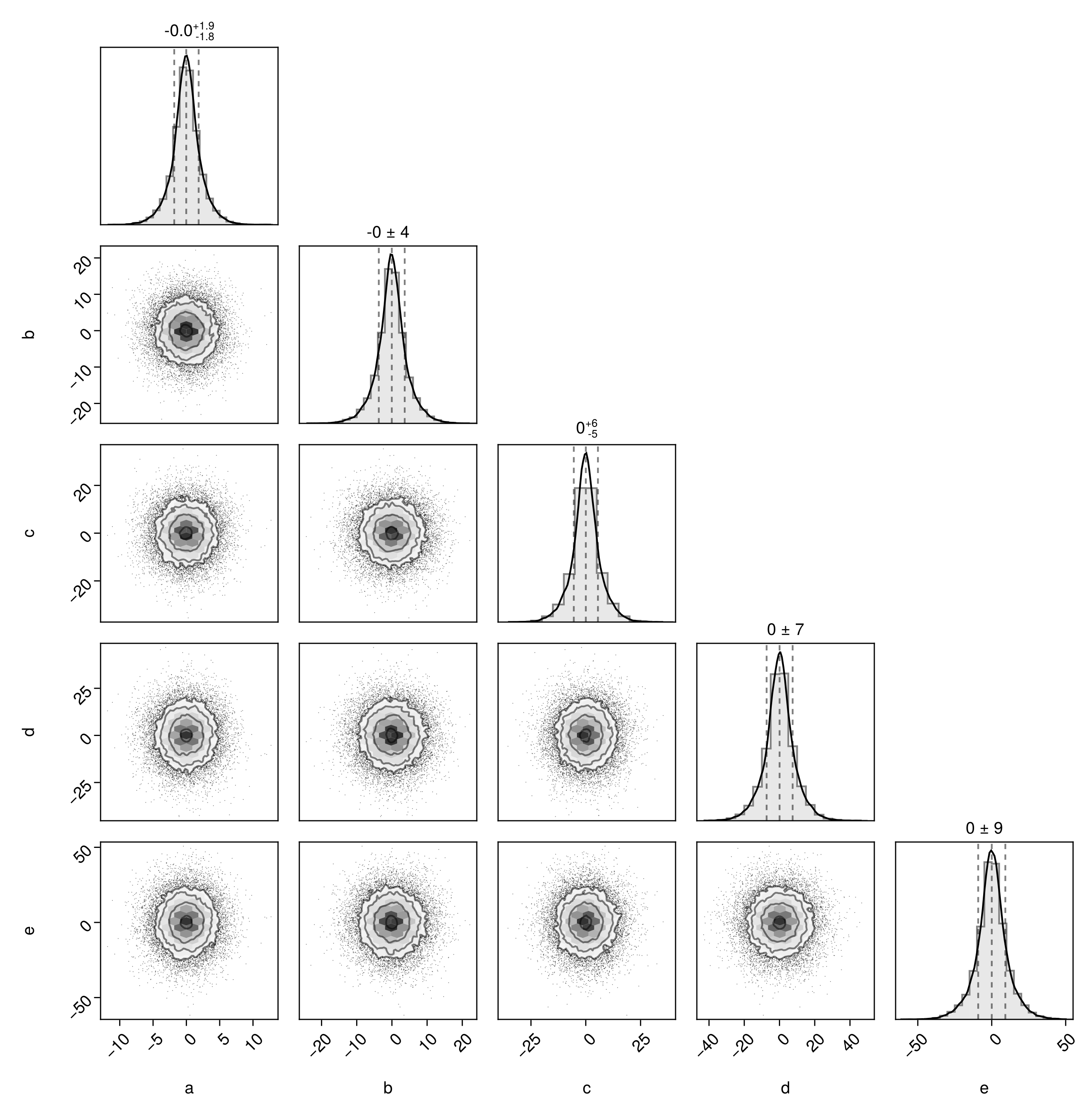
The labels are taken from the column names of the chains. You can modify them by passing in a dictionary mapping column names to strings, LaTeX strings, or Makie rich text objects.
Plotting individual chains separately
If you have multiple parallel chains and want to plot them in different colors, you can pass each one to pairplot:
pairplot(chn1[:,:,1], chn1[:,:,2], chn1[:,:,3])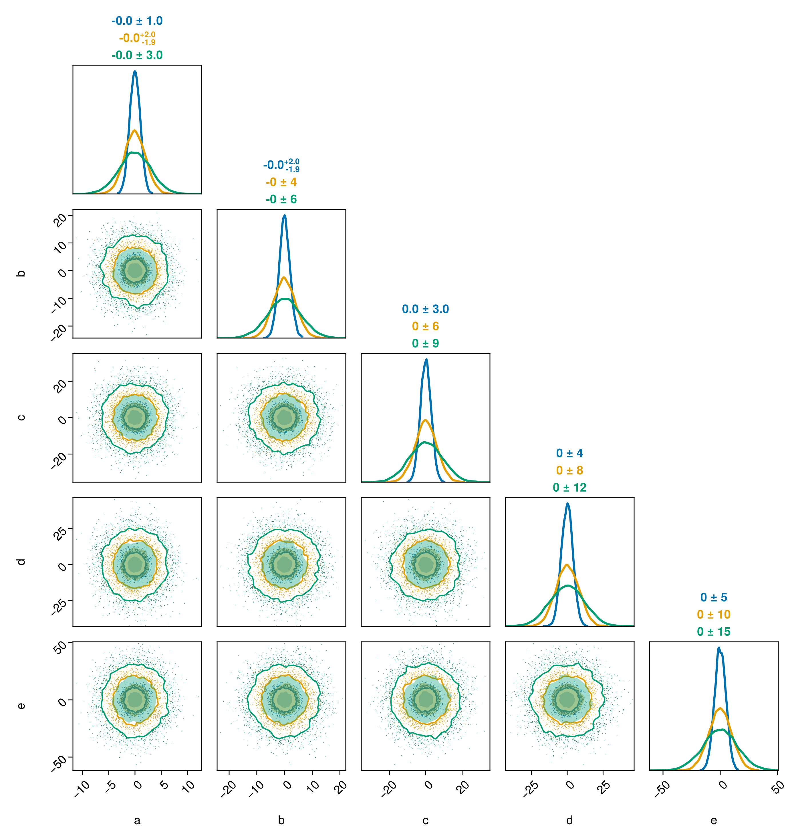
You can title the series indepdendently as well:
c1 = Makie.wong_colors(0.5)[1]
c2 = Makie.wong_colors(0.5)[2]
c3 = Makie.wong_colors(0.5)[3]

pairplot(
    PairPlots.Series(chn1[:,:,1], label="chain 1", color=c1, strokecolor=c1),
    PairPlots.Series(chn1[:,:,2], label="chain 2", color=c2, strokecolor=c2),
    PairPlots.Series(chn1[:,:,3], label="chain 3", color=c3, strokecolor=c3),
)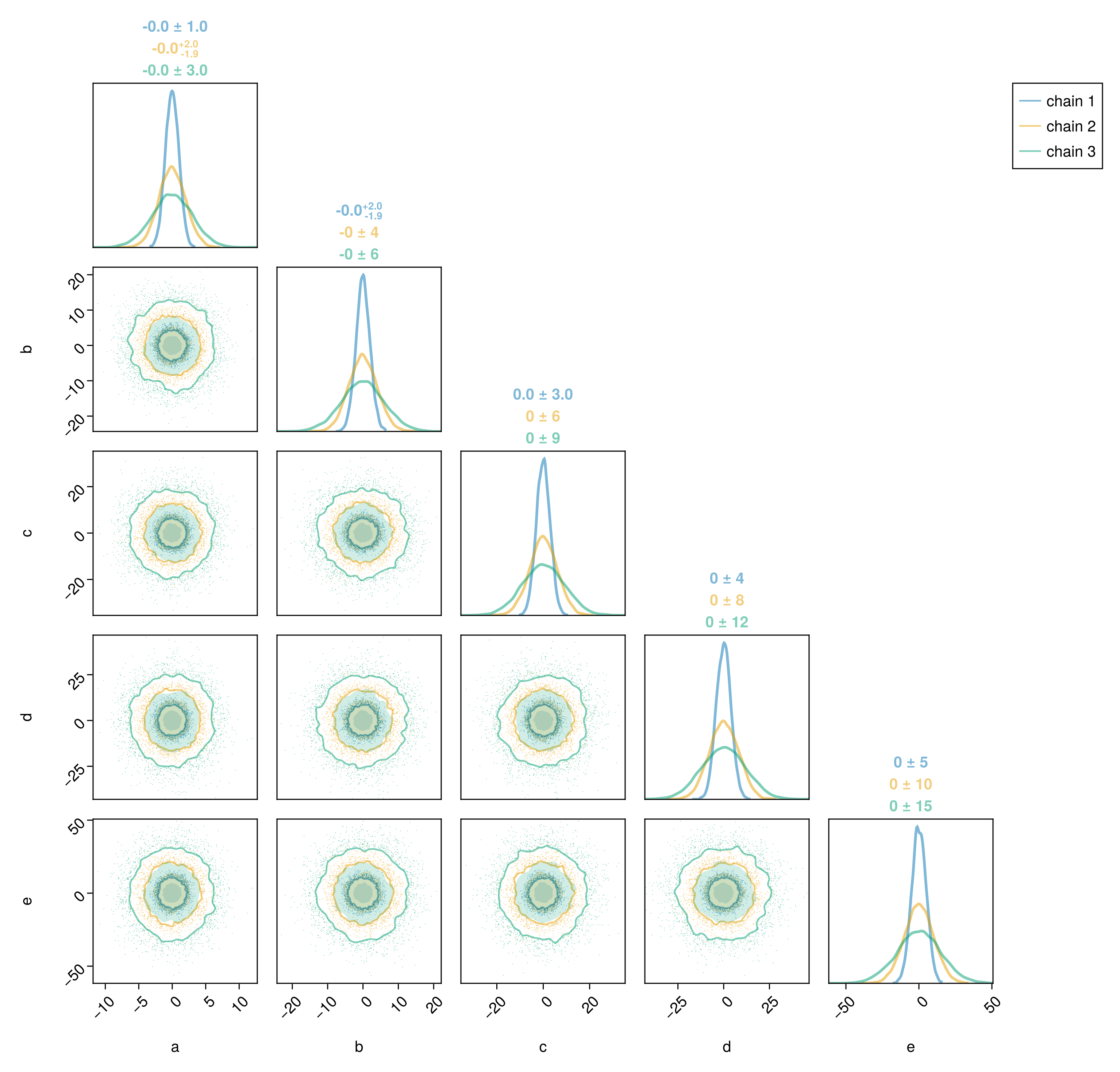
If your chains are well converged, then the different series should look the same.
Comparing the results of two simulations
You may want to compare the results of two simulations. Consider the following chains:
chn2 = Chains(randn(10000, 5, 1) .* [1 2 3 4 5], [:a, :b, :c, :d, :e])
chn3 = Chains(randn(10000, 4, 1) .* [5 4 2 1], [:a, :b, :d, :e]);
Chains MCMC chain (10000×4×1 Array{Float64, 3}):
Iterations = 1:1:10000
Number of chains = 1
Samples per chain = 10000
parameters = a, b, d, e
Use `describe(chains)` for summary statistics and quantiles.Just pass them all to pairplot:
pairplot(chn2, chn3)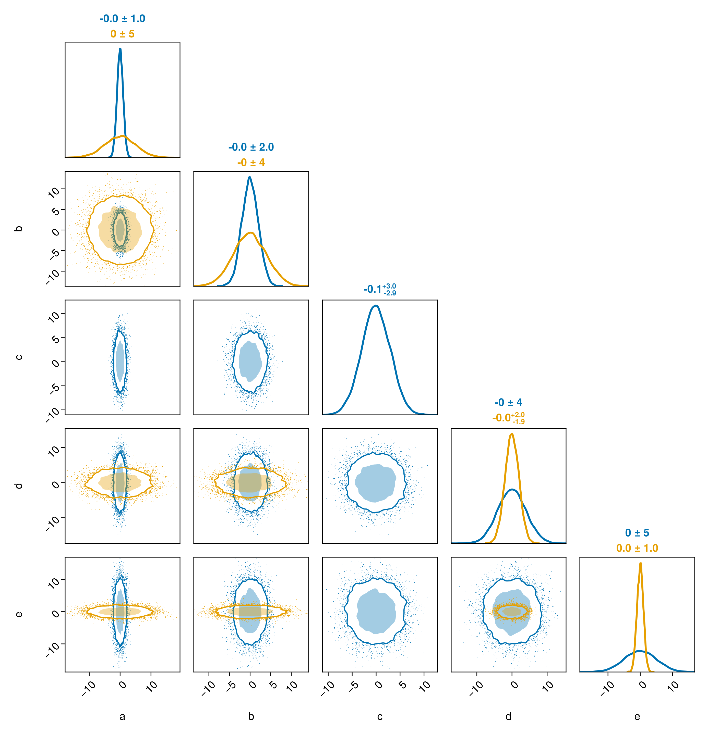
Note how the parameters of the chains do not have to match exactly. Here, chn2 has an additional variable not present in chn3.