Kepler solvers
Turning Keplerian elements into positions and velocities requires solving Kepler's equation, M = E − e·sin E, for the eccentric anomaly E. It is transcendental — there is no closed form for E in terms of M — so this one step is where essentially all of the arithmetic in a Keplerian model goes.
Orbital Mechanics & Astrodynamics derives it, along with the geometric meaning of the mean, eccentric and true anomalies, in Time Since Periapsis, Mean Anomaly, and Eccentric Anomaly and Circular and Elliptical Orbits. The unbound case, with sinh in place of sin, is in Hyperbolic Trajectories.
Worth knowing: the forward direction is trivial — M from E needs no solver at all. That asymmetry is why plotted orbit tracks are sampled in eccentric anomaly rather than in time; see Choosing epochs.
Which algorithm is used is selectable through the KeplerianApprox propagator:
orbitsolve(sys, epochs; method=KeplerianApprox(solver=PlanetOrbits.Markley()))Available solvers:
PlanetOrbits.Auto— the defaultPlanetOrbits.MarkleyPlanetOrbits.RootsMethodPlanetOrbits.HyperbolicHalley
Auto dispatches on eccentricity: Markley for e < 1, HyperbolicHalley for e > 1. Both are non-iterative or fixed-iteration, allocation-free, and always converge, which is what makes them safe defaults inside a sampler.
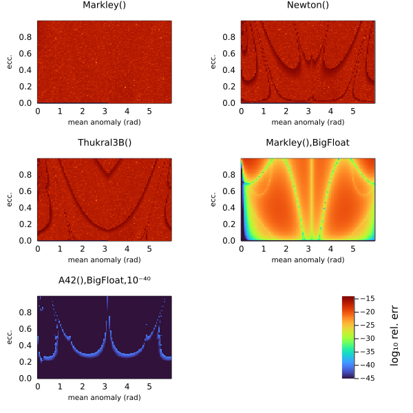
The Markley algorithm is a tweaked version of the one in AstroLib.jl. It is non-iterative and converges with less than 1e-15 relative error across the full range of e between 0 and 1. Because it is pure Julia there is no call overhead and no need for vectorization by hand.
RootsMethod wraps any algorithm from Roots.jl, which is the route to arbitrary precision — but note that Roots allocates, so it is not suitable for allocation-free hot loops.
The SIMD batch path
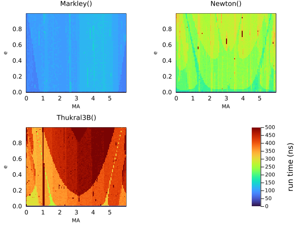
KeplerianApprox solves each hierarchy row across all epochs at once. For Float64 systems using Markley or Auto, that batch runs through branch-free kernels that vectorize across epochs — roughly 4× on AVX2, and agreeing with the scalar solver to ≤ 4e-15. Other element types (e.g. ForwardDiff Duals) and other solvers are compile-time routed to the scalar path.
Disable it with KeplerianApprox(simd=false) if you want to compare.
The hyperbolic solver
The hyperbolic Kepler equation M = e·sinh(H) − H is solved by a fixed iteration count of Halley steps from a closed-form starting guess. Unlike a Roots-based approach, this is allocation-free, so unbound orbits stay inside the same performance contract as bound ones. It carries its own implicit-differentiation rule, so ForwardDiff does not iterate through the solver.
High precision
Solve in arbitrary precision by building the system from BigFloat values and tightening the solver tolerance:
using Roots
import PlanetOrbits as PO

A = PO.Body(mass=big(1.0), name=:A)
b = PO.Body(mass=big(0.0), name=:b)
sys = PO.System((A, b), (PO.Orbit(b, about=A; a=big(1.2), e=big(0.1), ω=big(1.4)),))

method = KeplerianApprox(
    solver=PlanetOrbits.RootsMethod(Roots.Thukral5B(), rtol=1e-30, atol=1e-30))
radvel(orbitsolve(sys, big(59000.0); method), :b, :A)
Comparison